A Bayesian network is a directed graph in which each node is annotated with quantitative probability
information. This article covers the definition of a Bayesian network with a graphical representation,
the determination of independence between variables, and the problem of finding the probability
distribution of a set of query values given some observed events.
Published on Thu, Mar 5, 2020
Last modified on Sun, Sep 7, 2025
1006 words -
Page Source
Introduction
A Bayesian network is a directed graph in which each node is annotated with quantitative probability information. The full specification is as follows:
Each node corresponds to a random variable, which may be discrete or continuous.
A set of directed links or arrows connects pairs of nodes. If there is an arrow from node $X$ to node $Y$, $X$ is said to be a parent of $Y$. The graph has no directed cycles (and hence is a directed acyclic graph, or DAG).
Each node $X_i$ has a conditional probability distribution $P(X_i|Parents(X_i))$ that quantifies the effect of the parents on the node.
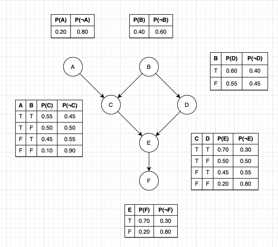
Example Bayesian Network
Semantics of a Bayesian network:
The network is a representation of a joint probability distribution
Encoding of a collection of conditional independence statements
Provided that $Parents(X_i) \subseteq { X_{i-1}, \ldots, X_1 }$
Conditional independence relations in bayesian networks
Steps to determine if two variables are conditionally independent
Draw the ancestral graph. Construct the “ancestral graph” of all variables mentioned in the probability expression. This is a reduced version of the original net, consisting only of the variables mentioned and all of their ancestors (parents, parents’ parents, etc.)
Moralize the ancestral graph by marrying the parents. For each pair of variables with a common child, draw an undirected edge (line) between them. (If a variable has more than two parents, draw lines between every pair of parents.)
Disorient the graph by replacing the directed edges (arrows) with undirected edges (lines).
Delete the givens and their edges. If the independence question had any given variables, erase those variables from the graph and erase all of their connections, too.
Given a query between two variables A, B
If the variables are disconnected, then they’re independent
If the variables are connected, then they’re dependent
If the variables are missing because they were a given, they’re independent
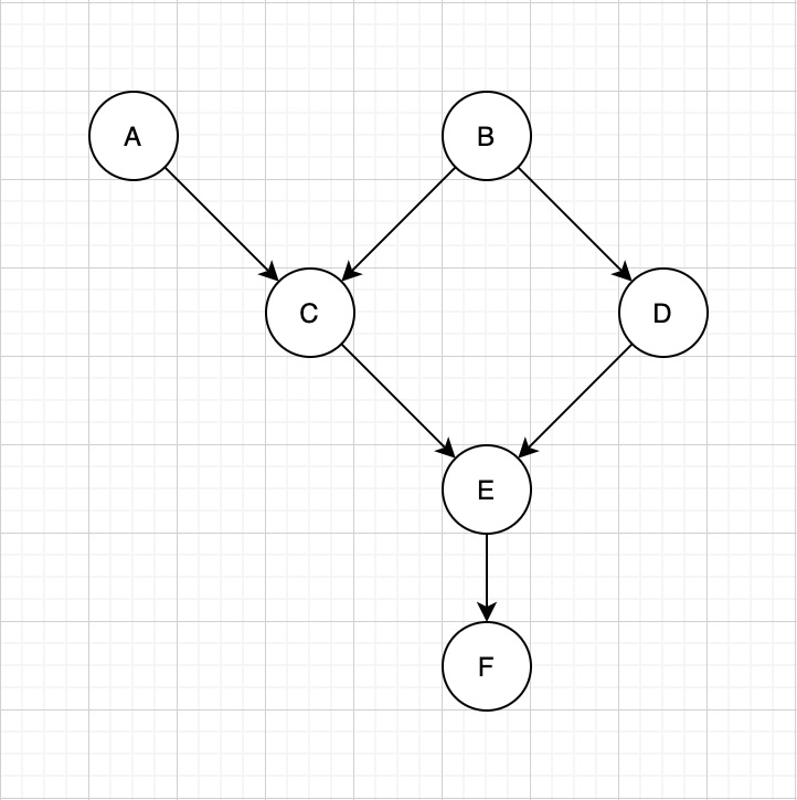
In the following example we skip step 1 and moralize the entire Bayesian network
Example Bayesian Network
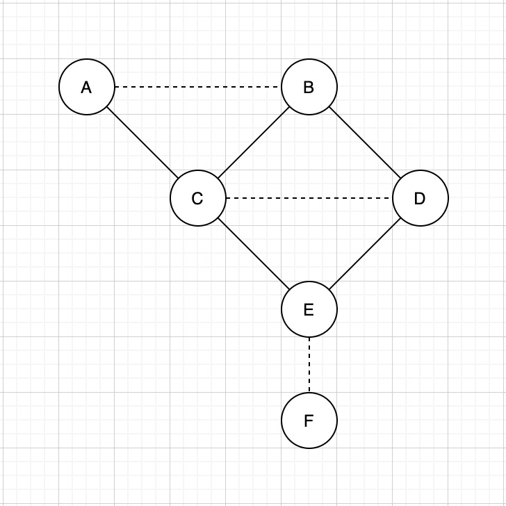
Example Bayesian Network Moralized
Some conditional independence queries ($\ci$ meaning conditionally independent of), delete the givens and their edges to check the connection between the query variables:
Is $A \ci B \given C$? No, there is a path A-B
Is $A \ci E \given C$? No, there is a path A-B-D-E
Is $A \ci E \given C,D$? Yes, there isn’t a path between A and E
Is $A \ci D \given C$? No, there is a path A-B-D
Is $B \ci E \given C$? No, there is a path B-D-E
Is $A \ci F \given C$? No, there is a path A-B-D-E-F
Is $A \ci F \given C,D$? Yes, there isn’t a path between A and F
Exact inference
Compute the posterior probability distribution for a set of query values given some observed event (set of evidence variables)
By enumeration
Any conditional probability can be computed by summing terms from the full joint distribution