In production systems, latency degradation rarely happens linearly. A service handling 5,000 requests per second with a 15ms response time might run smoothly all day, but an extra 5% traffic surge can suddenly spike tail latency from 15ms to 800ms.

This non-linear cliff is governed by queuing theory (the mathematical study of waiting lines).

(For foundational metrics, latency breakdowns, and resource utilization, see Performance Fundamentals .)

The Anatomy of Waiting: Why Queues Form

Consider a single worker thread (such as a Redis process, a Node.js event loop, or an isolated CPU core) where each task takes an average service execution time of $S = 10\text{ ms}$ (giving a maximum processing capacity of $\mu = \frac{1}{S} = 100\text{ req/s}$).

Suppose client traffic arrives at $\lambda = 50\text{ req/s}$, putting the worker at 50% utilization ($\rho = \frac{\lambda}{\mu} = 0.5$).

Clockwork vs. Random Bursts

In a perfectly synchronized system where requests arrive on a rigid, clockwork cadence (say, exactly one request every $20\text{ ms}$), the worker finishes each $10\text{ ms}$ task, rests for $10\text{ ms}$, and is always idle when the next request lands. Average queue wait is zero ($W_q = 0\text{ ms}$).

In real systems, requests arrive stochastically in random bursts (a Poisson arrival process). Because thousands of independent client browsers click buttons without coordinating with each other, arrivals naturally clump together in time. Even when average traffic is low (say, 50 req/s on average), 4 requests can randomly land within the exact same 5ms window, forcing 3 of them to wait in line.

What Happens When You Arrive: The Coin-Flip Model

When an incoming request arrives at a server with utilization $\rho = \frac{\lambda}{\mu}$, how many existing requests ($k$) will it find ahead of it?

Think of arriving at the server as a sequential coin-flip game where each flip lands on “Yes, a request is present” with probability $\rho$, and “No, the line stops here” with probability $1 - \rho$:

• $k = 0$ jobs (Server Idle): With probability $1 - \rho$, the worker is free. The request begins execution immediately with $0\text{ ms}$ queue wait.
• $k = 1$ job (Worker Busy): With probability $(1 - \rho)\rho$, exactly 1 job is executing. Due to the memoryless property of exponential service times, it still has an average of $S$ remaining. The incoming request waits $S$.
• $k = 2$ jobs (Worker Busy + 1 Queued): With probability $(1 - \rho)\rho^2$, 1 job is executing and 1 is queued. The incoming request waits $2 \times S$.
• $k = 3$ jobs (Worker Busy + 2 Queued): With probability $(1 - \rho)\rho^3$, 1 job is executing and 2 are queued. The incoming request waits $3 \times S$.

In general, for any count $k \ge 0$, the probability of finding exactly $k$ requests ahead in line is:

$$ P(N = k) = (1 - \rho)\rho^k $$

Summing the expected number of requests gives the average backlog ($L$):

$$ L = \sum_{k=0}^\infty k \cdot P(N = k) = (1 - \rho) \sum_{k=0}^\infty k \rho^k $$

To evaluate $\sum_{k=0}^\infty k \rho^k$, differentiate the standard geometric series with respect to $\rho$:

$$ \begin{aligned} \sum_{k=0}^\infty \rho^k &= \frac{1}{1 - \rho} \\ \frac{d}{d\rho} \left( \sum_{k=0}^\infty \rho^k \right) &= \frac{d}{d\rho} \left( \frac{1}{1 - \rho} \right) \\ \sum_{k=1}^\infty k \rho^{k-1} &= \frac{1}{(1 - \rho)^2} \\ \sum_{k=0}^\infty k \rho^k &= \frac{\rho}{(1 - \rho)^2} \end{aligned} $$

Substituting this series back into $L$:

$$ L = (1 - \rho) \cdot \frac{\rho}{(1 - \rho)^2} = \frac{\rho}{1 - \rho} $$

Multiplying that backlog by the average service execution time ($S$) yields the expected queue wait time ($W_q$):

$$ W_q = L \cdot S = \sum_{k=0}^{\infty} (k \cdot S) \cdot P(N = k) = \frac{\rho \cdot S}{1 - \rho} $$

Total server response time ($W$) is the queue wait plus execution time ($S$):

$$ W = W_q + S = \frac{\rho \cdot S}{1 - \rho} + S = \frac{S}{1 - \rho} $$

Worked Application ($\lambda = 50\text{ req/s}$, $S = 10\text{ ms}$)

Applying the formulas to our baseline worker handling $\lambda = 50\text{ req/s}$ with service time $S = 10\text{ ms}$ (service capacity $\mu = 100\text{ req/s}$, utilization $\rho = \frac{\lambda}{\mu} = 0.50$):

Evaluating the closed-form results:

• Expected Backlog: $L = \frac{0.50}{1 - 0.50} = \mathbf{1.0\text{ request}}$
• Expected Queue Wait: $W_q = 1.0 \times 10\text{ ms} = \mathbf{10\text{ ms}}$
• Total Latency: $W = \frac{10\text{ ms}}{1 - 0.50} = \mathbf{20\text{ ms}}$
• Little’s Law Check: $L = \lambda \cdot W = 50\text{ req/s} \times 0.020\text{ s} = \mathbf{1.0\text{ request}}$

The 50% Load Paradox: Why Does Latency Double?

Running a single-server queue at 50% CPU load ($\rho = 0.50$) does not mean near-zero queuing delay. Instead, average response time always doubles ($W = 2S$):

• 50% of the time, the server is completely idle, so the incoming request executes immediately ($\text{Wait} = 0$).
• 50% of the time, the server is busy processing a burst, where the expected wait for the backlog to clear is $2S$.

The overall average queue wait is the weighted combination of both states:

$$ W_q = \underbrace{(0.50 \cdot 0)}_{\text{Arrive when Idle}} + \underbrace{(0.50 \cdot 2S)}_{\text{Arrive when Busy}} = \mathbf{1.0 \cdot S} $$

Adding the task’s own execution duration ($S$) yields:

$$ W = W_q + S = 1.0S + 1.0S = \mathbf{2.0 \cdot S} $$

Even with 50% idle headroom, random Poisson arrival bursts cause enough temporary clumping that requests spend as much time waiting in line ($S$) as they do running on the CPU ($S$).

The Non-Linear Latency Penalty: The Hockey Stick Curve

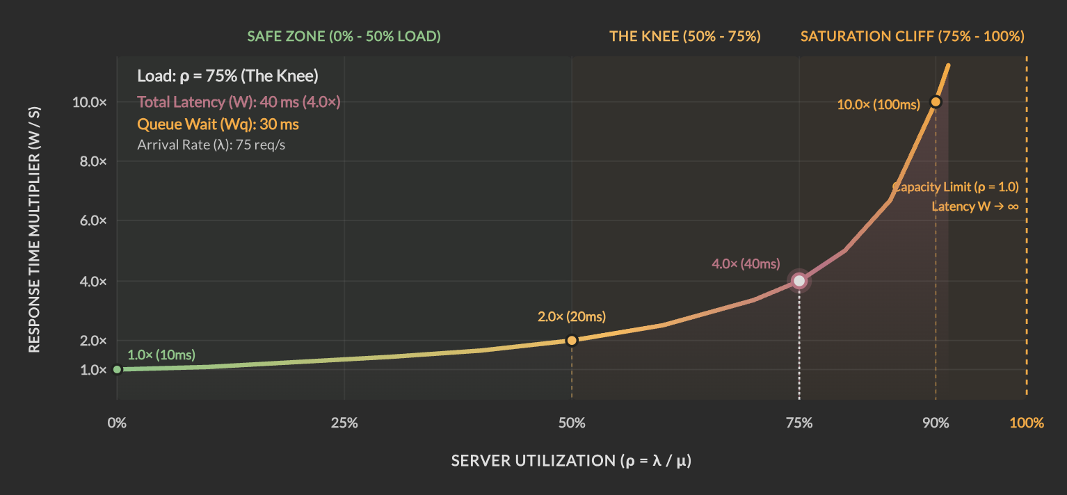
Because $W = \frac{S}{1 - \rho}$, response time scales with the hyperbolic multiplier $\frac{1}{1 - \rho}$. This causes latency to remain relatively flat across light and moderate loads before shooting upward asymptotically near capacity:

Applying Little’s Law strictly to the waiting queue buffer ($L_q = \lambda \cdot W_q$) with arrival rate $\lambda = \frac{\rho}{S}$ and queue wait $W_q = \frac{\rho \cdot S}{1 - \rho}$:

$$ L_q = \lambda \cdot W_q = \left(\frac{\rho}{S}\right) \cdot \left(\frac{\rho \cdot S}{1 - \rho}\right) = \frac{\rho^2}{1 - \rho} $$

Kendall’s Notation ($A/S/c$): A Universal Shorthand

Everything analyzed and simulated in the first half of this note describes an $M/M/1$ system: Memoryless arrivals, Memoryless service times, and 1 single worker.

To classify different queuing architectures, queuing theory uses Kendall’s Notation ($A/S/c$), introduced by David G. Kendall in 1953:

$$A / S / c$$

• $A$ (Arrival Process):
  • $M$ (Markovian / Memoryless): Random Poisson arrivals ($\lambda$).
  • $D$ (Deterministic): Fixed, clockwork intervals (e.g. cron schedule).
  • $G$ (General): Arbitrary arrival distribution.
• $S$ (Service Time Distribution):
  • $M$ (Exponential / Memoryless): Randomly distributed task execution times.
  • $D$ (Deterministic): Fixed, constant execution time for every job (e.g. exactly 10ms).
  • $G$ (General): Arbitrary or high-variance execution times (e.g. fast cache hits mixed with slow database scans).
• $c$ (Number of Parallel Servers): Count of independent worker threads or CPU cores.

With this vocabulary in place, we can explore two core deviations from the single-worker baseline:

1. Changing Service Distribution ($S \to G$): The variance penalty in an $M/G/1$ queue.
2. Changing Worker Count ($c \to N$): Multi-server pooling in an $M/M/c$ queue.

The Variance Penalty: Why Average Service Time Lies ($M/G/1$)

In the real world, execution times are rarely identical. Consider two different API services running on identical 100 req/s single-core workers at 80% utilization ($\lambda = 80\text{ req/s}, \mu = 100\text{ req/s}, S = 10\text{ ms}, \rho = 0.80$).

On a standard $M/M/1$ worker, the average queue wait time at 80% load is $40\text{ ms}$:

$$W_{q, M/M/1} = \frac{\rho \cdot S}{1 - \rho} = \frac{0.80 \cdot 10\text{ ms}}{1 - 0.80} = \mathbf{40\text{ ms}}$$

Now compare what happens when service execution times change:

• Service A (Deterministic): Every request is a fixed-size cryptographic token validation that takes exactly $10\text{ ms}$.
• Service B (High Variance): 90% of requests are fast $1\text{ ms}$ cache lookups, but 10% are heavy $91\text{ ms}$ unindexed database queries. Average service time is still exactly $10\text{ ms}$ ($(0.90 \times 1\text{ ms}) + (0.10 \times 91\text{ ms}) = 10\text{ ms}$).

In a single-worker queue, waiting in line is caused by two separate sources of randomness: when requests arrive (arrival jitter) and how long requests take to execute (service jitter). Each source contributes roughly half of the total queue delay.

What happens to average queue wait time ($W_q$)?

• In Service A, execution time is fixed at exactly $10\text{ ms}$, eliminating service jitter entirely. With half of the system’s randomness gone, average queue wait time drops in half to $20\text{ ms}$ ($0.5\times$ of baseline $M/M/1$).
• In Service B, execution jitter explodes ($1\text{ ms}$ cache hits mixed with $91\text{ ms}$ table scans), trapping fast requests behind heavy queries and inflating queue wait time to $200\text{ ms}$ ($5\times$ baseline $M/M/1$, $10\times$ higher than Service A).

Why does Service B suffer $10\times$ worse queuing delay when both services have the exact same 80% utilization and identical $10\text{ ms}$ average execution time?

Head-of-Line Blocking

Because requests share a single FIFO queue, whenever one of those 91ms heavy queries enters execution, it holds the worker hostage. Dozens of fast 1ms requests that arrive right behind it get trapped waiting in line.

The Pollaczek–Khinchine (P-K) Formula

To quantify execution time spread, we use the Coefficient of Variation ($C_v$), defined as the standard deviation of service time ($\sigma$) divided by the mean service time ($S$):

$$C_v = \frac{\sigma}{S}$$

• $C_v = 0$ (Deterministic): Every task takes the exact same duration ($\sigma = 0$).
• $C_v = 1$ (Exponential / $M/M/1$): Standard random variance where $\sigma = S$.
• $C_v > 1$ (High Variance / Bimodal): Fast tasks mixed with heavy tail outliers ($\sigma > S$).

The mathematical relationship between service time variance and queue wait time is governed by the Pollaczek–Khinchine (P-K) formula ($M/G/1$):

$$ W_q = \underbrace{\left(\frac{\rho \cdot S}{1 - \rho}\right)}_{\text{Baseline } M/M/1 \text{ Wait}} \times \underbrace{\left(\frac{1 + C_v^2}{2}\right)}_{\text{Variance Multiplier}} $$

The variance multiplier term scales queue waiting time directly:

1. Deterministic Execution ($C_v = 0$): $$\frac{1 + 0}{2} = 0.5 \implies W_q = 0.5 \times 40\text{ ms} = \mathbf{20\text{ ms}} \quad (\text{Service A})$$ When every task takes the exact same time, queue wait time is cut in half.
2. Exponential Execution ($C_v = 1$): $$\frac{1 + 1^2}{2} = 1.0 \implies W_q = 1.0 \times 40\text{ ms} = \mathbf{40\text{ ms}} \quad (\text{Baseline } M/M/1)$$
3. High-Variance Execution ($C_v = 3$): $$\frac{1 + 3^2}{2} = \frac{1 + 9}{2} = 5.0 \implies W_q = 5.0 \times 40\text{ ms} = \mathbf{200\text{ ms}} \quad (\text{Service B})$$ A high-variance distribution inflates queue wait time by $5\times$ over baseline and $10\times$ over deterministic execution.

Systems Engineering Takeaway: Isolate Variance

The P-K formula proves mathematically why fast, interactive workloads must never share an unpartitioned FIFO queue with slow, unpredictable batch operations:

• Separate Queues by Workload: Route fast queries to read replicas and heavy analytical scans to a dedicated offline worker pool.
• Enforce Strict Execution Timeouts: Reject or preempt queries that exceed $3\sigma$ of expected service time.
• Chunk Heavy Jobs: Break large $100\text{ms}$ jobs into ten $10\text{ms}$ sub-tasks to bound $C_v \to 0$.

The Power of Resource Pooling: 1 Queue vs. Many Queues ($M/M/c$)

Now consider scaling up from 1 worker to $c$ parallel workers handling an aggregate arrival rate $\lambda$.

Compare two different architectural patterns handling 400 req/s across 4 workers:

• Design A (4 Isolated Single-Worker Queues, $4 \times M/M/1$): Incoming traffic is split (e.g. by round-robin DNS or static hashing). Each worker has its own private queue and handles 100 req/s on 1 core ($\rho = 0.80$, 80% load).
• Design B (1 Pooled Shared Queue, $1 \times M/M/4$): All 400 req/s enter a single shared FIFO queue. Whichever worker finishes its job first immediately pulls the next request from the queue.

Why Pooling Wins: The Erlang C Formula

In Design A, a sudden cluster of 4 requests hitting Worker 1 creates a severe queue backlog on that single node, even while Worker 3 sits completely idle. Isolated queues lead to simultaneous queue delays and idle waste.

In Design B, a worker is never idle when there is work waiting to be done.

Mathematically, the probability that an incoming request finds all $c$ workers busy and must wait in line is given by the Erlang C formula (see Erlang C derivation for the complete birth-death Markov chain proof):

$$P(\text{Wait} > 0) = C(c, a) = \frac{\frac{a^c}{c!} \frac{1}{1 - \rho}}{\sum_{k=0}^{c-1} \frac{a^k}{k!} + \frac{a^c}{c!} \frac{1}{1 - \rho}}$$

where $a = \frac{\lambda}{\mu} = c \cdot \rho$ is traffic intensity in Erlangs.

The average queue wait time across $c$ pooled workers is:

$$W_q = \frac{C(c, a) \cdot S}{c(1 - \rho)}$$

Notice the factor of $c$ in the denominator: pooling $c$ workers cuts average queue wait time by roughly a factor of $c$ at the exact same overall utilization $\rho$.

Worked Comparison: 4 Isolated Queues vs. 1 Shared Queue

Evaluating our 4-worker cluster handling $400\text{ req/s}$ at 80% utilization ($\lambda = 400\text{ req/s}, S = 10\text{ ms}, c = 4, \rho = 0.80$):

• Design A ($4 \times M/M/1$): $$W_{q, A} = \frac{0.80 \cdot 10\text{ ms}}{1 - 0.80} = \mathbf{40\text{ ms}}$$
• Design B ($1 \times M/M/4$): With traffic intensity $a = 4 \times 0.80 = 3.2$ Erlangs, the Erlang C probability is $C(4, 3.2) \approx 0.596$ (59.6% chance of finding all cores busy): $$W_{q, B} = \frac{0.596 \cdot 10\text{ ms}}{4 \cdot (1 - 0.80)} = \frac{5.96\text{ ms}}{0.80} = \mathbf{7.5\text{ ms}}$$

Simply pooling the 4 cores to pull from a single shared queue reduces average queue wait from $40\text{ ms}$ to $7.5\text{ ms}$ (over $5\times$ faster) with identical total throughput, identical hardware, and identical 80% CPU load.

The Capacity Planning Mental Model

Subtracting execution time ($S$) from total response time ($W = \frac{S}{1 - \rho}$) isolates the pure queue wait multiplier:

$$W_q = W - S = \frac{S}{1 - \rho} - S = \left(\frac{\rho}{1 - \rho}\right) \cdot S$$

When sizing server clusters or diagnosing latency regressions, translate target utilization ($\rho$) directly into task durations of queue wait ($W_q = \text{Multiplier} \times S$):

Summary & Systems Engineering Rules of Thumb