

Benchmarking production infrastructure is difficult. It is easy to run a naive closed-loop load test, receive a clean report claiming a “p99 latency of 12ms at 5,000 req/s”, and deploy to production only to suffer catastrophic tail latency spikes under a fraction of that traffic.
The exact same illusion happens in generative AI systems: running an LLM benchmark with tools like
inference-perf
or
aiperf
using a fixed 128-token prompt might report a “p99 Time to First Token (TTFT) of 30ms”, only for the server to suffer multi-second TTFT delays and GPU KV-cache memory exhaustion when production traffic sends real-world 4,000-token conversational prompts.
Most benchmarks lie not because the hardware is broken, but because the test was designed without grounding in queuing theory. When a benchmark ignores the mechanics of waiting lines, it falls into critical measurement traps like Coordinated Omission, masks queue buildup behind self-throttling virtual users, and tests an artificial synthetic workload that bears no resemblance to production traffic.
Accurate capacity planning is an empirical science. It requires a disciplined problem statement, rigorous workload characterization, and open-loop measurement tooling.
To ground these principles in production practice, this guide follows two running architectures side by side:
- Classical Web & Database Backends: CPU-bound worker processes, connection-pooled relational databases, and disk/memory page caches.
- Generative AI Inference Clusters: GPU tensor accelerators, continuous batching iteration schedulers, and VRAM KV-cache memory pools.
While their physical hardware constraints differ (CPU cores and transactional locks vs. GPU tensor cores and High-Bandwidth Memory), both obey the exact same queuing mechanics and saturation mathematics.
(For foundational formulas and queue derivations, see Performance Fundamentals and Queuing Theory for Systems Engineers .)
The Performance Problem Statement Method
Before launching any load testing tool, you must define the experimental parameters of the test. Running a benchmark without a formal problem statement is like running a randomized stress test: it generates CPU heat, but produces numbers you cannot safely use for sizing clusters or verifying Service Level Agreements (SLAs).
A complete performance problem statement establishes five core dimensions:
Test Goals & Environmental Controls
A complete benchmark specification establishes explicit experimental controls:
- Explicit Test Objective: Load tests serve three distinct purposes:
- Capacity Discovery: Finding the maximum throughput ($\lambda_{\text{knee}}$) the system can sustain before crossing the operational knee ($\rho \approx$ 75%) into hyperbolic queue delays (or discovering maximum concurrent token rates before TTFT and TPOT diverge in LLM serving).
- SLA / Regression Gating: Verifying that a new release satisfies strict tail latency bounds in CI/CD pipelines ($P_{99} \le 25\text{ ms}$ for web APIs, or $\text{TTFT}_{99} \le 200\text{ ms}$ and $\text{TPOT}_{99} \le 25\text{ ms/token}$ for streaming LLM endpoints).
- Saturation & Resilience Mapping: Deliberately pushing the system past 100% capacity to verify graceful degradation (circuit breakers, shedding load with HTTP 429/503, KV-cache sequence preemption, and avoiding out-of-memory crashes).
- Anticipated Failure Modes: Identify what resource will exhaust first across infrastructure layers: compute core saturation, database connection starvation, socket/port exhaustion (
TIME_WAIT), GC Stop-the-World pauses, GPU VRAM KV-cache block exhaustion, or High-Bandwidth Memory (HBM) bus saturation during autoregressive decode. - Strict Environment Isolation: Never run the load generator tool on the same physical host or virtual machine as the target server. Ensure network bandwidth between the load generator and server is at least $10\times$ higher than peak expected test bandwidth. In multi-GPU inference deployments, ensure Tensor Parallelism (TP) communication uses dedicated NVLink / NVSwitch fabrics rather than congested PCIe bridges.
Baseline Service Floor ($S$) & Latency Multipliers
Before measuring contention under heavy traffic, measure the baseline execution duration ($S = W_0$) under near-zero load ($\rho <$ 5%, single request at a time). This value represents the physical execution floor of your code, database queries, and compute kernels (uncontended prefill latency $S_{\text{prefill}}$ and decode step latency $S_{\text{decode}}$).
Setting arbitrary millisecond SLA targets (such as “P99 must be under 50ms”) is dangerous without knowing the underlying execution floor ($S$):
- Too Loose (Hiding Collapse): If an API endpoint has an uncontended baseline of $S = 2\text{ ms}$, a $50\text{ ms}$ threshold allows a $25\times$ latency multiplier:
$$ \frac{W}{S} = \frac{50\text{ ms}}{2\text{ ms}} = 25, \quad \frac{1}{1 - \rho} = 25 \implies \rho = \mathbf{0.96} $$
This allows the system to reach 96% load ($\rho = 0.96$), operating deep in the saturation cliff on the verge of complete collapse while alerts stay green.
- Physically Impossible: If a database query has a baseline execution time of $S = 30\text{ ms}$, a $50\text{ ms}$ SLA is mathematically impossible even at moderate 50% load ($W = 2S = 60\text{ ms}$).
Instead of arbitrary numbers, frame percentile SLAs as multipliers of the baseline service duration ($S$), bounded by an OS jitter noise floor ($t_{\text{floor}} \approx 1\text{ to } 2\text{ ms}$ for sub-millisecond endpoints):
$$ \begin{aligned} P_{50} &\le 1.5 \times S \\ P_{95} &\le 3.0 \times S \\ P_{99} &\le \max(4.0 \times S, t_{\text{floor}}) \end{aligned} $$
These multipliers map directly to practical operational zones in pooled systems:
- $P_{50} \le 1.5 \times S$ (Median): Below 50% load, the server is idle more than half the time ($\text{Wait} = 0$). Median requests start almost immediately, keeping $P_{50}$ close to the uncontended floor ($1.0 \times S$ to $1.5 \times S$).
- $P_{95} \le 3.0 \times S$ (High Percentile): Absorbs Poisson arrival bursts and execution variance ($C_v$). At 67% load ($\rho = 0.67$), mean response time is $W = \frac{S}{1 - 0.67} = 3.0S$.
- $P_{99} \le 4.0 \times S$ (The Operational Knee): At the target sizing knee ($\rho = 0.75$), multi-server pooling and deterministic execution keep 99th percentile response time within $4.0 \times S$.
- Sub-Millisecond Baseline Clamping: For fast cache lookups ($S = 0.2\text{ ms}$), a strict $4.0 \times S$ threshold ($0.8\text{ ms}$) will be violated by routine Linux CFS kernel scheduling jitter and network interrupts. Clamping to $\max(4.0 \times S, 2\text{ ms})$ prevents false SLA alarms on microsecond workloads.
When latency departs from linear scaling and smoothly climbs such that $P_{99} > 10 \times S$, queuing theory proves the system has breached the knee and entered the saturation cliff ($\rho >$ 90%). (Isolated, bimodal tail spikes at low utilization indicate discrete runtime pauses like GC pauses or DB lock flushes rather than queue capacity exhaustion).
Workload Characterization: Modeling Production Reality
The most common reason load tests fail to predict production outages is synthetic workload distortion. If you benchmark an API endpoint by sending millions of identical static requests, the entire dataset fits in CPU L1/L2 caches and database buffer pools, achieving an artificial $S = 0.5\text{ ms}$. In production, real traffic touches millions of distinct keys, hitting cold NVMe storage and triggering multi-millisecond disk reads.
Similarly, in generative AI systems, benchmarking an LLM inference server with fixed 128-token prompts completely masks memory fragmentation, prefix cache eviction, and the asymmetric compute profiles of real workloads.
To produce meaningful capacity data, characterize the workload across four core dimensions:
- Execution Variance ($C_v$) and Polymorphism: As proven by the Pollaczek–Khinchine (P-K) formula, queue waiting time scales directly with service time variance ($W_q \propto \frac{1 + C_v^2}{2}$). In web backends, homogeneous queries ($C_v \approx 0$) artificially cut reported wait times in half compared to high-variance production lookups ($C_v \ge 1.0$). In LLM serving, variable prompt/output token lengths cause head-of-line blocking and KV-cache fragmentation that uniform test payloads completely hide.
- Access Skew and Cache Locality (Zipfian Distributions): Production traffic follows power-law distributions where roughly 80% of requests target the top 20% of keys. Sampling keys with a calibrated Zipfian distribution ($s \approx 0.8$ to $1.1$) produces realistic database buffer pool hit rates and authentic GPU prefix-cache reuse in VRAM (e.g. RadixAttention in vLLM / SGLang).
- Operational Phase Ratios (Compute vs. Memory Bandwidth): Backend performance shifts dramatically between read-only paths and write-heavy paths with lock contention. Similarly, LLM inference alternates between compute-bound matrix-matrix multiplication (prefill GEMM) and memory-bandwidth-bound matrix-vector streaming (decode GEMV). Workloads must calibrate the exact input/output token ratio matching production traffic.
- Temporal Arrival Dynamics & Continuous Batching: Clockwork arrivals eliminate queuing jitter, whereas real traffic exhibits Poisson memoryless arrival bursts. In LLM continuous batching engines, sudden bursts of compute-dense prefill requests interleave with ongoing decode loops, injecting severe tail latency jitter into streaming token generation (Time Per Output Token, TPOT).
The Benchmark Specification & Execution Protocol
A reliable benchmark requires strict experimental protocol. Without structured execution phases, transient startup anomalies will contaminate steady-state measurements.
The 4-Phase Lifecycle & Steady-State Distributions
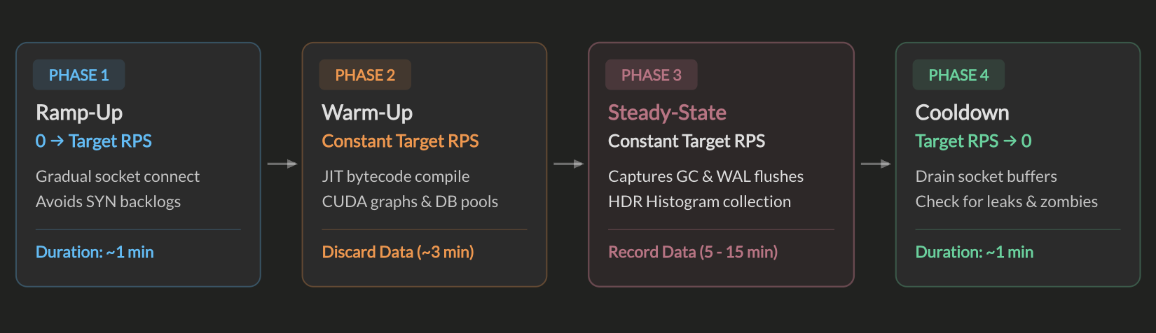
A complete benchmark specification defines four sequential lifecycle phases:
- Phase 1: Ramp-Up Window: Gradually scale arrival rate $\lambda$ from 0 to the target operating point over 30 to 60 seconds. Jumping instantly to high loads creates artificial TCP SYN backlogs and socket allocation panics that do not reflect normal traffic growth.
- Phase 2: Warm-Up & JIT Priming (Discard Metrics): Run the target load for 2 to 5 minutes without recording latency metrics. This allows V8/JVM JIT compilation, database buffer pool warming (
shared_buffers), connection pool handshakes, and inference engine CUDA graph capture (pre-allocating the PagedAttention KV-cache pool) to complete. - Phase 3: Steady-State Measurement: Record high-resolution latency histograms over 5 to 15 minutes under constant rate $\lambda$, long enough to capture recurring GC cycles, database write checkpoints, and WAL flushes.
- Phase 4: Cooldown (Drain & Health Check): Reduce traffic to zero over 30 to 60 seconds to drain in-flight socket buffers cleanly (preventing false
ECONNRESETerrors) and verify there are no memory leaks, unclosed connection leaks, or zombie processes.
During steady-state measurement, a single arithmetic average (mean) collapses the distribution, hiding severe tail spikes behind fast-path requests:
Rate-Stepped Sweeps & Statistical Replication
Never run a load test at a single arbitrary throughput number. To discover the operational knee, execute a stepped rate sweep across a series of steady-state windows:
$$ \lambda = 1\text{k} \to 2\text{k} \to 4\text{k} \to 6\text{k}\text{ req/s} $$
Plotting average response time ($W$) and $P_{99}$ against arrival rate ($\lambda$) reveals the exact throughput threshold where latency departs from the uncontended floor and enters the hyperbolic saturation curve.
To ensure statistical confidence and prevent cloud noise from corrupting results:
- Multi-Run Replication ($N \ge 3$): Run an odd number of identical, independent trials ($N = 3$ or $N = 5$) with complete ramp-up and warm-up cycles.
- Coefficient of Variation ($C_v$) Stability Check: Calculate the relative standard deviation across runs under identical target load ($C_v = \frac{\sigma}{\mu}$). If $C_v \le$ 3% (or under 10% on shared virtualized cloud instances), the benchmark environment is statistically stable. If $C_v >$ 10%, noisy neighbors or hypervisor steals are contaminating the measurement: discard the run set and re-test on isolated hardware.
- Merge Raw HDR Histograms (Avoid Averaging Percentiles): Averaging percentile metrics across runs (such as taking the arithmetic mean of three $P_{99}$ numbers) is mathematically invalid because percentiles are non-linear quantile distributions. Export raw HdrHistogram logs from each trial and merge them into a single unified distribution to compute the true ensemble $P_{99}$ and $P_{99.9}$.
- Noise Calibration for Pareto Evaluation: The same multi-run distribution is the right input for setting the noise parameters used in Pareto frontier evaluation (discussed in The Pareto Frontier in LLM Inference Serving ). Once you have $N$ independent runs for a given configuration, you can compute the per-metric standard deviation $\sigma$ and coefficient of variation $C_v$ from the ensemble. These directly calibrate the noise band ($\sigma_{\text{noise}} \approx C_v$) and give a principled lower bound for the minimum percentage improvement threshold: an improvement must exceed the $C_v$ of the metric to be distinguishable from run-to-run variance. Using empirically measured distributions rather than a fixed hardcoded percentage makes both parameters traceable and environment-specific.
- Minimum for Baseline Floor ($S$) vs. Ensemble for Contended Load ($\rho$): When measuring uncontended baseline execution time ($S = W_0$), use the minimum observed latency across light-load trials to filter out OS interrupts. When measuring contended load ($\rho \approx$ 75%), evaluate the merged ensemble distribution across trials to capture typical queuing behavior.
Open-Loop vs. Closed-Loop Load Models
Choosing between an open-loop and a closed-loop load generator determines whether benchmark results will reflect production reality:
- Closed-Loop Model (Self-Throttling): The rate of new requests is strictly tied to the server’s response time. If the server slows down, virtual users wait longer, automatically reducing the request arrival rate. While appropriate for modeling internal batch workers pulling from a single bounded queue, closed-loop testing must never be used for public web APIs or microservices: self-throttling virtual users mask queuing cliffs and cannot trigger production-like queue exhaustion.
- Open-Loop Model (Independent Arrivals): Requests arrive at rate $\lambda(t)$ completely independent of server response time, accurately modeling public HTTP APIs, mobile clients, and multi-tenant systems. If the server pauses, incoming requests continue arriving at rate $\lambda$, filling the queue buffer and faithfully reproducing production tail latency spikes.
Coordinated Omission: The Silent Benchmark Killer
The most widespread measurement flaw in production load testing is Coordinated Omission, a term coined by Gil Tene in his presentation How NOT to Measure Latency .
When a load generator coordinates its request dispatches with the server’s response rate, it hides long server pauses and reports artificially optimistic latency percentiles. Consider an intended arrival rate of 10 requests per second (one request every $100\text{ ms}$):
- At $t = 0.0\text{s}$, the tool sends Request 1. The server responds in $1\text{ ms}$. Recorded latency: $1\text{ ms}$.
- At $t = 0.1\text{s}$, the tool sends Request 2. The server suffers a Garbage Collection pause or database table lock and stalls for $10.0\text{ seconds}$.
- During that 10-second stall, the load tester blocks synchronously, waiting for Request 2’s response before sending Request 3.
- The 100 other requests that should have been dispatched during those 10 seconds were never sent.
When the naive tool computes percentiles across recorded requests, it reports $P_{50} = 1\text{ ms}$ and $P_{99} = 10,000\text{ ms}$ (dismissing the stall as a single isolated 1% outlier).
In reality, 100 production clients arrived during those 10 seconds and waited in socket buffers ($9.9\text{s}$, $9.8\text{s}$, …, $0.1\text{s}$). 98% of users experienced multi-second delays, and the true median was $5.0\text{ seconds}$. The naive benchmark coordinated with the server’s pause, omitting the backlog of suffering requests.
Fixing Coordinated Omission: Schedule Delay Correction
To eliminate Coordinated Omission, modern load testing tools use open-loop, rate-corrected measurement:
- Intended Dispatch Timestamp: Pre-calculate the exact intended schedule time ($t_{\text{scheduled}}$) for every request.
- Schedule Delay Tracking: Measure total response time ($L_{\text{true}}$) starting from the intended schedule time rather than the actual socket write time:
$$ \begin{aligned} L_{\text{true}} &= t_{\text{response}} - t_{\text{scheduled}} \\ &= \underbrace{(t_{\text{dispatch}} - t_{\text{scheduled}})}_{\text{Schedule Delay}} + \underbrace{(t_{\text{response}} - t_{\text{dispatch}})}_{\text{Server Latency}} \end{aligned} $$
- Accumulated Backlog Accounting: If the server stalls, every request accumulating in the queue receives its full schedule penalty, faithfully reporting the true production tail percentiles ($P_{99}$, $P_{99.9}$).
Tool Configuration: Why Defaults Mislead
Load generators do not automatically eliminate Coordinated Omission. Many popular benchmarking tools operate in closed-loop mode by default, placing the burden of correct configuration on the benchmark developer:
wrk2: Inwrk2’s specification , passing the intended throughput rate with-R <rate>pre-calculates scheduled dispatch times and tracks schedule delay via HdrHistograms. Note thatwrk2operates over a fixed pool of-cpersistent TCP connections: it measures true schedule delay over established channels, but does not open new sockets to test OS-level TCP backlog queues (somaxconn).Locust: In Locust’s task execution architecture , eachHttpUserexecutes tasks sequentially in a greenlet loop (send$\to$wait$\to$sleep), reducing request velocity whenever the server stalls.vegeta&aiperf/inference-perf: Built natively around open-loop execution: Vegeta’s pacer engine (lib/pacer.go) dispatches requests using a strict monotonic timer (-rate=<rps>). Always configure--max-workers=0(unlimited) when characterizing long stalls, ensuring Vegeta does not hit its default 10,000 worker threshold and block dispatch. Similarly,inference-perfandaiperfgenerate requests following a stochastic Poisson arrival process to benchmark LLM continuous batching systems.
When developing benchmarks, always verify whether your tool measures raw completion latency ($t_{\text{response}} - t_{\text{dispatch}}$) or true schedule-corrected latency ($t_{\text{response}} - t_{\text{scheduled}}$). Running closed-loop tools with default options masks the severe queuing backlogs you are attempting to characterize.
Mapping Real Systems to Queuing Models
Every component in a distributed infrastructure maps directly to a specific queuing model with distinct capacity constraints:
Single-Threaded Event Loops ($M/M/1$)
- Real-World Examples: Redis server, Node.js V8 main loop, NGINX single-worker process.
- Internal Mechanics: A single OS thread loops continuously, popping commands from an incoming socket FIFO buffer.
- Capacity Dynamics: Single-threaded execution has zero lock contention or context-switching overhead. However, a single long-running operation (such as an unindexed Redis
KEYS *scan or a massive synchronous JSON parse in Node.js) stalls the entire thread. This triggers immediate Pollaczek–Khinchine Head-of-Line blocking, forcing all subsequent lightweight requests to queue behind the slow job.
Connection-Pooled Relational Databases ($M/M/c / K$)
- Real-World Examples: PostgreSQL or MySQL fronted by connection poolers like PgBouncer or HikariCP.
- Internal Mechanics: The database manages a fixed pool of $c$ backend worker processes (e.g. $c = 32$ connections). When all $c$ connections are busy, incoming application queries wait in a client-side FIFO queue capped at buffer capacity $K$.
- Capacity Dynamics: Governed strictly by Little’s Law ($N = \lambda \cdot W$). If average query execution time jumps from $5\text{ ms}$ to $50\text{ ms}$ due to database lock contention, sustaining $\lambda = 1,000\text{ queries/s}$ requires increasing active concurrent connections from 5 to 50:
$$ N = \lambda \cdot W = 1,000\text{ req/s} \times 0.050\text{ s} = \mathbf{50\text{ connections}} $$
If the pool is capped at $c = 32$, the connection pool exhausts immediately ($K$ reached) and subsequent queries fail with connection timeout errors.
Multi-Worker HTTP Microservices ($G/G/c$)
- Real-World Examples: Go HTTP servers with goroutine pools, Java Spring Tomcat thread pools, Python Gunicorn worker pools.
- Internal Mechanics: Inbound HTTP requests exhibit arbitrary payload sizes and variable compute times ($G$) dispatched across $c$ worker threads or CPU cores ($c$).
- Capacity Dynamics: Governed by Erlang C resource pooling. Pooling $c$ cores behind a shared queue drastically reduces queuing delay compared to isolated single-server pipelines, allowing the service to absorb short traffic bursts without degrading tail latency.
LLM Continuous Batching Engines ($G/G/1\text{ (GPU)}$ with Iteration Scheduling)
- Real-World Examples: vLLM, SGLang, TensorRT-LLM, Hugging Face TGI.
- Internal Mechanics: The GPU accelerator acts as a high-throughput server processing continuous iteration batches. Requests enter a two-phase lifecycle: (1) compute-bound prefill evaluated in parallel chunks, and (2) memory-bandwidth-bound decode iterated token-by-token. The engine dynamically multiplexes active requests into continuous batch steps, bounded by the GPU VRAM KV-cache capacity pool ($K$).
- Capacity Dynamics: Governed by KV-cache block limits and HBM memory bandwidth. When active concurrent sequences exhaust available KV blocks ($K$), incoming requests wait in an external admission queue ($W_q$). When a burst of long prompts arrives, compute-heavy prefill operations interleave with ongoing decode loops, causing severe tail spikes in Time Per Output Token (TPOT).
Distributed Inference Clusters & Disaggregated Queuing ($G/G/c$)
- Real-World Examples:
llm-d(Kubernetes-native distributed inference orchestration), vLLM / SGLang multi-node clusters with Gateway API Inference routing. - Internal Mechanics: Multi-node inference clusters scale out by disaggregating execution phases and pooling GPU workers:
- Prefill-Decode (PD) Disaggregation: Decouples the single heterogeneous queue into separate specialized worker pools: compute-dense prefill workers ($M/G/c_{\text{prefill}}$) and memory-bandwidth-dense decode workers ($M/G/c_{\text{decode}}$), passing the generated KV cache over high-speed RDMA interconnects. This drives execution variance on decode workers down ($C_v \approx 0$), eliminating prefill-induced TPOT jitter.
- Prefix-Cache-Aware Routing: Evaluates incoming prompt hashes to route requests directly to the node hosting matching KV cache blocks, turning $S_{\text{prefill}} = 500\text{ ms}$ into $S_{\text{prefill}} = 5\text{ ms}$ and dramatically shrinking in-flight cluster concurrency ($L = \lambda \cdot W$).
- Capacity Dynamics: Governed by Erlang C multi-server pooling and KV cache transfer bandwidth. Centralized inference-aware gateways prevent request clumping across nodes, ensuring all worker GPUs operate symmetrically near the 75% operational knee without localized queue blowouts.
Production Capacity Planning Checklist
Apply these five sizing principles to translate empirical benchmark results into production infrastructure sizing:
- Measure Baseline Service Floor ($S = W_0$): Measure median response time ($P_{50}$) under light load ($\rho <$ 5%) with network transit latency subtracted ($S = W_{\text{uncontended}} - t_{\text{RTT}}$). This physical execution floor establishes the reference baseline for all queuing contention.
- Identify Maximum Knee Throughput ($\lambda_{\text{knee}}$): Execute an open-loop stepped rate sweep (
wrk2 -R) in increments of 10% load. Identify $\lambda_{\text{knee}}$ where tail response time first departs from linear scaling ($P_{99} \le 3.0 \times S$). - Size Cluster Nodes for Peak Traffic ($c_{\text{nodes}}$): Size node count so that the cluster operates safely at $\rho_{\text{target}} \le$ 75% during peak traffic demand ($\lambda_{\text{peak}}$), preserving 25% idle capacity to absorb stochastic Poisson bursts:
$$ \begin{aligned} c_{\text{nodes}} &= \left\lceil \frac{\lambda_{\text{peak}}}{\lambda_{\text{knee, node}}} \right\rceil \\ &= \left\lceil \frac{\lambda_{\text{peak}}}{0.75 \cdot \lambda_{\text{max, node}}} \right\rceil \end{aligned} $$
- Size Resource Pools with Little’s Law Safety Upper-Bounds ($N_{\text{pool}} = \lambda_{\text{peak}} \cdot W_{P_{99}}$): While Little’s Law ($L = \lambda W$) mathematically governs expected means, sizing concurrency pools to peak worst-case duration ($W_{P_{99}}$) provides an essential engineering safety buffer against resource exhaustion cascades during traffic bursts:
- Database Connection Pools: If an API handles $\lambda = 2,000\text{ req/s}$ with a peak $P_{99}$ query duration of $40\text{ ms}$ ($0.040\text{ s}$), the pool must contain at least $N_{\text{pool}} = 2,000 \cdot 0.040 = \mathbf{80\text{ active connections}}$ to avoid queue drop errors.
- LLM Inference KV-Cache Memory Pools: If an inference cluster receives $\lambda = 50\text{ req/s}$ with an average request turnaround duration of $W = 4.0\text{ s}$ (prefill + decode), GPU VRAM must allocate enough PagedAttention memory blocks to hold $N_{\text{sequences}} = 50 \cdot 4.0 = \mathbf{200\text{ concurrent sequences}}$.
- Synchronize Defensive Client Timeouts: Set client-side timeouts based on high quantiles ($3 \times P_{90}$ or $P_{99.9}$). Never allow client timeouts to exceed the server’s queue retention window. When a client abandons a request, the server must immediately cancel the in-flight context (e.g. Go
context.WithTimeoutor gRPC deadline propagation) to avoid wasting compute cycles on abandoned work.
Summary Matrix
| Performance Dimension | Naive Load Testing (Anti-Pattern) | Systems Engineering Practice |
|---|---|---|
| Problem Definition | Running a tool without baseline service time floor $S$. | Formal Problem Statement: capacity discovery, SLA gating, or failure mapping. |
| Workload Model | Static single-key requests with homogeneous duration ($C_v \approx 0$). | Zipfian key distribution with production read/write ratio and execution variance ($C_v$). |
| Execution Protocol | Immediate 0 to max load, measuring during cold startup. | 4-Phase Protocol: Ramp-up, JIT/Pool Warm-up, Steady-State, Stepped Rate Sweeps. |
| Load Generation Model | Closed-loop virtual users (self-throttling, which masks saturation). |
Open-loop arrival generation (
wrk2
,
vegeta
).
|
| Omission Correction | Ignores schedule delay (reports fake $1\text{ms}$ median during stalls). | Calculates true latency $L_{\text{true}} = t_{\text{received}} - t_{\text{scheduled}}$. |
| Target Sizing Point | Sizing at 95% utilization to save hosting costs. | Sizing at the operational knee ($\rho \approx$ 70% to 75%) with 25% burst headroom. |
| Pool Sizing | Guessing arbitrary thread and connection pool limits. | Little’s Law safety sizing: $N_{\text{pool}} = \lambda_{\text{peak}} \cdot W_{P_{99}}$. |
| Tooling Approach | Naive closed-loop scripts or uncorrected virtual-user loops. |
Open-loop tools:
wrk2
,
vegeta
, and
aiperf
/
inference-perf
.
|
This note was co-authored in pair programming with Antigravity (Agy) .