
There is no single best configuration for an LLM inference server. A single scalar is a lossy projection: collapsing competing objectives into one number hides the underlying trade-offs across different workloads.
(For foundational queuing theory, latency breakdowns, and classical service metrics, see Performance Fundamentals . For benchmark design, see Benchmarking & Capacity Planning .)
The Limits of a Single Number
Serving an LLM is an inherently multi-objective problem with conflicting physical constraints:
- Maximizing throughput requires saturating the GPU with large batches, which increases queueing delay.
- Minimizing Time to First Token ($\text{TTFT}$) requires small batches and idling compute during decode.
- Minimizing Inter-Token Latency ($\text{ITL}$) requires protecting active decode streams, which steals cycles from prompt prefill.
In practice, benchmarks and leaderboards reduce performance to a single number in two common ways:
- Reporting an isolated headline metric: Ranking engines purely by Peak Throughput ($\text{TPS}$), ignoring that peak throughput drives latency past interactive service level objectives (SLOs).
- Collapsing metrics into a composite score: Minimizing a single synthetic aggregate (for example, $0.5 \cdot \text{TTFT} + 0.5 \cdot \text{TPOT}$) using arbitrary preset weights.
Both approaches hide the underlying trade-offs:
- Peak throughput alone says nothing about tail latency (P99 $\text{TTFT}$ / $\text{TPOT}$) under concurrency.
- Isolated latency numbers (such as low median $\text{TTFT}$ at concurrency 1) say nothing about throughput capacity.
- A composite score winner is only optimal for the specific weight ratio picked before tuning began, while creating incentives to overfit toward that single benchmark score.
When a workload changes, the dropped trade-off shape is precisely what you need.
Why Scalarization Cannot Recover the Frontier
The instinct when facing multiple objectives is to fold them into one. This is called scalarization, and the most common form is the weighted sum. Given objectives $f_1, f_2, \dots, f_k$, you minimize a weighted aggregate:
$$ g(\mathbf{x}) = \sum_{i=1}^{k} w_i f_i(\mathbf{x}), \quad \sum_{i=1}^{k} w_i = 1 $$
Pick weights, solve the single-objective problem, get one point. Change the weights, solve again, get another point. In theory, sweeping the weights traces out the trade-off surface.
In practice it does not always. The weighted sum can only reach points on the convex part of the frontier. If the frontier curves the other way, if it is concave in objective space, then no weight vector reaches points in that region. Those points are called unsupported or non-dominated but non-supported, and a weighted sum misses them by construction. This is a well-documented limitation of weighted-sum scalarization: for a concave front it cannot approximate the whole trade-off, no matter how finely you sweep the weights.
Two very different operating points can produce the identical weighted score, while balanced solutions in concave regions remain unreachable through linear weighting.
Other scalarizations exist, such as Tchebycheff (Chebyshev) scalarization and $\varepsilon$-constraint methods . Unlike linear weighted sums, $\varepsilon$-constraint methods (optimizing one primary metric such as throughput while constraining others like $\text{TTFT}_{P99} \le 1.2\text{s}$) can reach non-convex regions of the frontier.
Industrial serving platforms often pair both approaches: exploring the full multi-objective frontier during offline benchmarking, and applying $\varepsilon$-constrained rules at deploy time when an automated Continuous Delivery (CD) pipeline must commit a single concrete configuration to a Kubernetes cluster.
The frontier remains the minimal object that contains the complete trade-off surface. A single scalar solve collapses it into a single decision.
The Frontier Is the Artifact
Formally, a configuration $\mathbf{x}$ maps to an objective vector $F(\mathbf{x}) = [f_1(\mathbf{x}), f_2(\mathbf{x}), \dots, f_k(\mathbf{x})]$ over the configuration space $\mathcal{X}$.
A configuration $\mathbf{x}_A$ dominates $\mathbf{x}_B$ ($\mathbf{x}_A \succ \mathbf{x}_B$) if it is no worse in every objective and strictly better in at least one:
$$ \mathbf{x}_A \succ \mathbf{x}_B \iff \forall i, \quad f_i(\mathbf{x}_A) \le f_i(\mathbf{x}_B) \quad \text{and} \quad \exists j, \quad f_j(\mathbf{x}_A) < f_j(\mathbf{x}_B) $$
The Pareto frontier $\mathcal{P}^*$ is the set of all configurations that no other configuration dominates:
$$ \mathcal{P}^* = { \mathbf{x} \in \mathcal{X} \mid \nexists \mathbf{x}’ \in \mathcal{X} : \mathbf{x}’ \succ \mathbf{x} } $$
Every point on the frontier is a legitimate answer. The frontier is the reportable artifact, and no point on it outranks another. The point you pick depends on the workload, which is exactly why the set, not the point, is what you keep.
Keeping the frontier means keeping a collection of trials or configurations, each with its full vector of objective values. It means resisting the pressure to pick one and discard the rest. The reason is practical: the right operating point changes with the workload, and you do not know the workload in advance. A batch ETL job and a real-time voice agent face the same hardware but want opposite corners of this plane. The frontier preserves both choices.
The Frontier Is Derived, Not Stored
Manually tuning serving parameters (such as batch sizes, sequence concurrency, memory limits, and chunked prefill) across a combinatorial grid is intractable when every benchmark trial consumes real GPU time. Hyperparameter optimization (HPO) frameworks automate this black-box search: multi-objective algorithms (like NSGA-II , the Non-dominated Sorting Genetic Algorithm II by Deb et al., 2002) iteratively suggest candidate configurations to navigate competing trade-offs without requiring an explicit analytical model of the GPU execution engine. (While mechanistic profiling like roofline analysis and trace profiling identifies whether bottlenecks are compute- or memory-bound, black-box HPO automates search across the resulting parameter interactions.)
How do these frameworks represent the resulting trade-off surface? Tools like Optuna and Google Vizier do not store a static Pareto frontier in their database schemas. Instead, both persist every trial as a raw objective vector, and the frontier is derived on demand via a dominance filter whenever queried.
What Optuna Actually Stores
In Optuna, a multi-objective study is created with a list of directions, one per objective:
import optuna

def objective(trial: optuna.Trial):
    max_num_batched_tokens = trial.suggest_categorical(
        "max_num_batched_tokens", [512, 1024, 2048, 4096, 8192]
    )
    max_num_seqs = trial.suggest_int("max_num_seqs", 16, 256, step=16)
    gpu_memory_utilization = trial.suggest_float("gpu_memory_utilization", 0.80, 0.95, step=0.05)
    enable_chunked_prefill = trial.suggest_categorical("enable_chunked_prefill", [True, False])

    tps, p99_ttft, p99_tpot = run_benchmark(
        max_num_batched_tokens=max_num_batched_tokens,
        max_num_seqs=max_num_seqs,
        gpu_memory_utilization=gpu_memory_utilization,
        enable_chunked_prefill=enable_chunked_prefill,
    )

    # Maximize TPS, minimize TTFT P99, minimize TPOT P99
    return tps, p99_ttft, p99_tpot

sampler = optuna.samplers.NSGAIISampler(population_size=50)
study = optuna.create_study(
    directions=["maximize", "minimize", "minimize"],
    sampler=sampler
)
study.optimize(objective, n_trials=100)
Each finished trial carries a full values tuple (here, the three metrics) alongside its params. That tuple is what gets persisted. There is no stored frontier. The moment you access
study.best_trials
, Optuna recomputes the non-dominated subset by comparing every trial’s value vector against every other:
pareto_trials = study.best_trials  # recomputed, not read from storage
print(f"Discovered {len(pareto_trials)} Pareto-optimal configurations:")
for trial in pareto_trials:
    print(f"Trial #{trial.number}: Values (TPS, TTFT, TPOT) = {trial.values}")
    print(f"  Params: {trial.params}")
plot_pareto_front
does the same thing under the hood, filtering the full trial history for non-dominated points before rendering. The frontier is a query over the population, never a persisted object. The design decision is to keep every evaluation and treat the frontier as an ephemeral filter on top of it.
Google Vizier follows the identical architectural model. Completed Vizier trials persist full Measurement metric dictionaries. The service does not store a static frontier object; calling study.optimal_trials() triggers the listOptimalTrials RPC to compute non-dominated points on demand.
Both tools treat the frontier as an ephemeral query over complete historical trials. The cost of persisting the raw metric vectors is negligible, ensuring any future workload requirement can derive a fresh Pareto frontier without re-running benchmarks.
Benchmarks Are Noisy: Building a Noise-Aware Evaluator
The tools above treat every trial measurement as ground truth. In practice, infrastructure benchmarks are not deterministic, and applying raw Pareto dominance to noisy numbers produces a polluted frontier.
Noise Bands and Minimum Improvement Thresholds
Standard multi-objective optimization algorithms (such as NSGA-II) operate on clean, deterministic numbers. In production infrastructure, benchmarks are noisy. Network jitter, noisy neighbors on shared hosts, variable prompt lengths, and GPU thermal throttling mean that two identical benchmark trials rarely report identical metrics.
As discussed in Benchmarking & Capacity Planning for Systems Engineers , the first line of defense is running multiple trials per configuration and taking medians to dampen measurement variance.
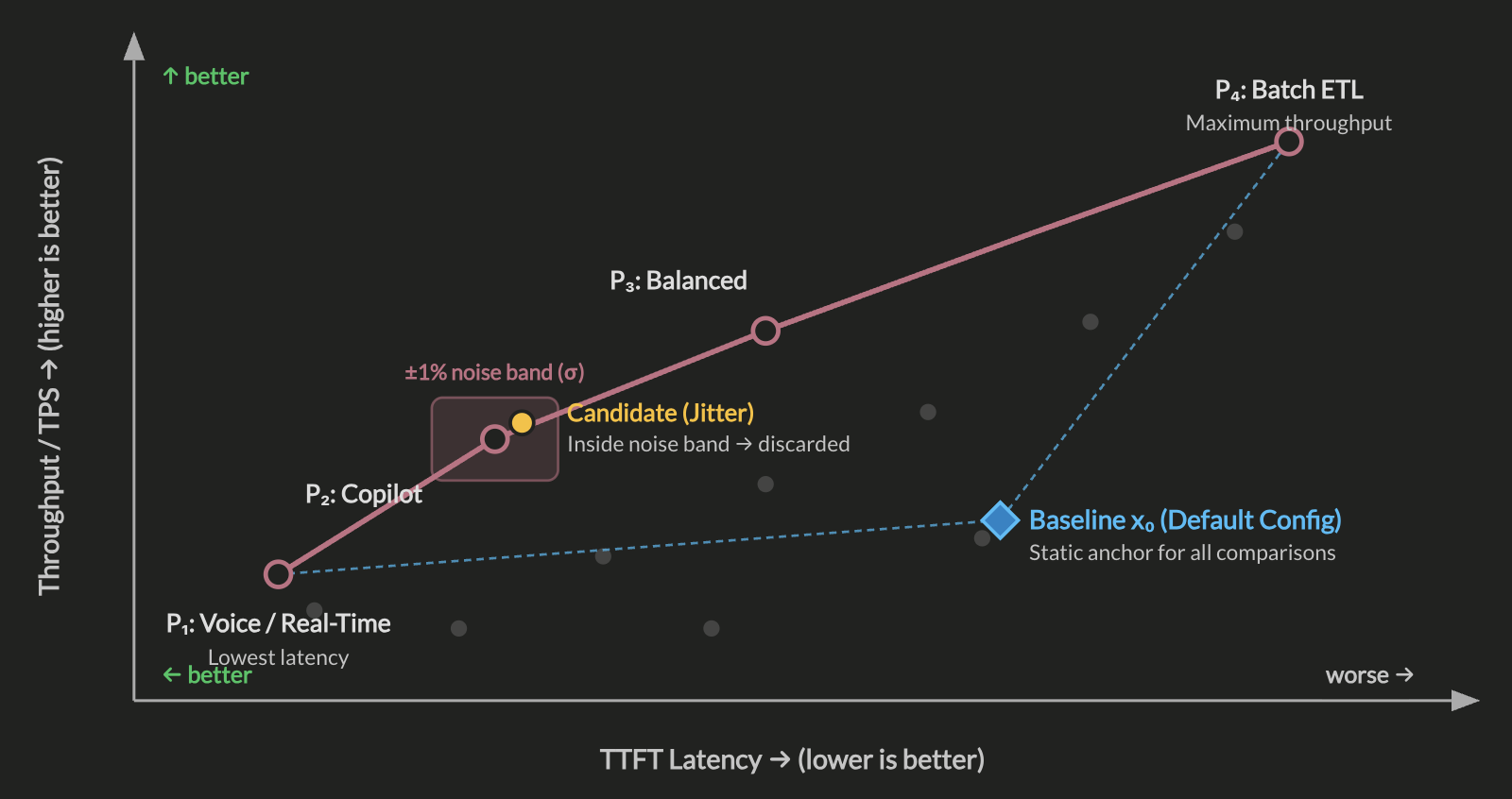
When evaluating production candidates at scale, raw Pareto dominance tests need practical bounds. Consider a configuration where throughput is effectively unchanged, but $\text{TTFT}$ improves by 0.5%:
- If 0.5% is within normal run-to-run jitter, treating it as a new Pareto point pollutes the frontier with measurement noise.
- Conversely, if $\text{TTFT}$ improves by 6% while throughput fluctuates by a negligible 0.3%, the configuration represents a real engineering improvement and belongs on the frontier.
To separate true frontier advances from environmental noise, real-world evaluation pipelines layer two complementary parameters on top of the dominance query:
- A Noise Band Vector ($\vec{\sigma}_{\text{noise}}$): Defines the equivalence threshold for environmental jitter per metric. Because tail metrics (like $\text{TTFT}_{P99}$) exhibit higher variance ($C_v$ of 10%–20%) than mean throughput or deterministic memory usage ($C_v$ of 1%–2%), noise thresholds are naturally configured per-objective rather than as a single global scalar.
- A Minimum Percentage Improvement Vector ($\vec{\delta}_{\text{min}}$): Defines the bar for a meaningful win on each objective. A candidate only claims a spot on the frontier if it outperforms an existing point by at least $\delta_{\text{min}, j}$ on at least one objective while remaining within the noise band or better across all other objectives.
Formally, a candidate $\mathbf{x}_A$ dominates $\mathbf{x}_B$ under practical $(\vec{\sigma}, \vec{\delta})$-filtering when:
$$ \forall i, \quad f_i(\mathbf{x}_A) \le f_i(\mathbf{x}_B) \cdot (1 + \sigma_{\text{noise}, i}) \quad \text{and} \quad \exists j, \quad f_j(\mathbf{x}_A) \le f_j(\mathbf{x}_B) \cdot (1 - \delta_{\text{min}, j}) $$
(for minimization objectives).
Wrapping standard HPO trial stores with a deterministic evaluator that enforces noise equivalence and minimum improvement thresholds keeps the resulting Pareto frontier sparse, robust, and actionable for engineering decisions.1
Grounding Improvements Against a Fixed Baseline
A subtle failure mode in relative comparison rules is accumulated drift (caused by the intransitivity of noisy equivalence).
Consider what happens if candidate evaluation only compares points pairwise and sequentially against the latest admitted candidate:
- Candidate $A$ is admitted as the best initial point.
- Candidate $B$ is measured. It sits within the noise tolerance band of $A$ (differing by less than $\sigma_{\text{noise}}$), so it is admitted as an equivalent peer.
- Candidate $C$ is measured. It sits within the noise tolerance band of $B$ (differing by less than $\sigma_{\text{noise}}$), so it is also admitted.
Chaining sequential relative comparisons creates a random walk. Over dozens of iterations, the frontier can drift toward configurations that are noticeably worse than $A$, because each step passed a small, relative tolerance check ($A \approx B$ and $B \approx C$, but $A \not\approx C$).
To prevent drift, percentage improvements must be grounded against a fixed, reproducible baseline configuration $\mathbf{x}_0$ (such as the default production configuration with all tuning levers disabled):
$$ \Delta_i(\mathbf{x}) = \frac{f_i(\mathbf{x}) - f_i(\mathbf{x}_0)}{f_i(\mathbf{x}_0)} $$
Grounding deltas to an unmoving anchor $\mathbf{x}_0$ provides three practical guarantees:2
- No cumulative drift: The improvement threshold is anchored to a static reference, preventing the scale from degrading across sequential trials.
- Stable scale across iterations: A 5% $\text{TTFT}$ reduction in trial 50 represents the exact same physical latency improvement as a 5% reduction in trial 1.
- Clear production reporting: Every point on the final Pareto frontier can state its exact delta relative to the baseline (e.g.
+35%$\text{TPS}$,-15%$\text{TTFT}$,+2GBVRAM vs. default).
The Moving Baseline in Continuous Integration
In production infrastructure, runtime components evolve: engine releases (such as upgrading vLLM or SGLang), CUDA updates, and new FlashAttention kernels improve performance over time.
If $\mathbf{x}_0$ is frozen from an older software release, a framework upgrade can cause an unoptimized configuration to register a false 10% tuning win. Conversely, if $\mathbf{x}_0$ is updated on every commit, historical frontier points become difficult to compare across git history.
Production tuning pipelines address this with two conventions:
- In-Study Re-Benchmarking: The baseline configuration $\mathbf{x}_0$ is re-benchmarked within the active CI run on the exact same cluster nodes, ensuring all candidate comparisons reflect the current software and hardware state.
- Version-Scoped Metadata: Every frontier artifact is tagged with environmental metadata (
engine_version,cuda_version,gpu_driver). Comparisons across versions compare the new baseline $\mathbf{x}_0^{(v+1)}$ against the prior baseline $\mathbf{x}_0^{(v)}$ before evaluating parameter changes.
The walkthrough below traces how raw mathematical dominance compares against a noise-aware $(\sigma, \delta)$-filter grounded to baseline $\mathbf{x}_0$ across four candidate evaluation scenarios:
Filtering in Practice: Custom Dominance on Optuna and Vizier
Neither
study.best_trials
nor Vizier’s listOptimalTrials RPC applies a noise band or minimum improvement threshold. Both use strict mathematical dominance, so a 0.1% improvement is enough to admit a new frontier member.
To get noise-aware filtering, skip the built-in frontier query and apply your own dominance function over the raw completed trial list:
import optuna

def noise_aware_dominates(a_values, b_values, sigmas, deltas):
    """Return True if candidate a pairwise dominates candidate b under (sigma, delta)-filtering."""
    # a must not be worse than b beyond metric noise tolerance on any objective
    no_worse = all(
        a <= b * (1 + s)
        for a, b, s in zip(a_values, b_values, sigmas)
    )
    # a must achieve a meaningful win over b on at least one objective
    meaningful_win = any(
        a <= b * (1 - d)
        for a, b, d in zip(a_values, b_values, deltas)
    )
    return no_worse and meaningful_win

def noise_aware_pareto(trials, sigmas, deltas, slo_bounds=None):
    """Derive the non-dominated Pareto frontier enforcing SLOs and (sigma, delta)-filtering."""
    # 1. Hard SLO feasibility filter (feasibility precedes dominance)
    viable_trials = []
    for t in trials:
        if slo_bounds:
            meets_slos = all(
                bound is None or val <= bound
                for val, bound in zip(t.values, slo_bounds)
            )
            if not meets_slos:
                continue
        viable_trials.append(t)

    # 2. Pairwise (sigma, delta)-dominance pruning
    dominated = set()
    for i, t_a in enumerate(viable_trials):
        for j, t_b in enumerate(viable_trials):
            if i != j and noise_aware_dominates(t_a.values, t_b.values, sigmas, deltas):
                dominated.add(j)
    return [t for i, t in enumerate(viable_trials) if i not in dominated]

# Query all completed trials and apply custom filter
# Objectives: [-TPS (minimize), TTFT_P99 (ms), TPOT_P99 (ms)]
all_trials = [t for t in study.trials if t.state == optuna.trial.TrialState.COMPLETE]

# Tail latency (TTFT P99) has higher noise (15%) than throughput (2%)
sigmas = (0.02, 0.15, 0.10)
deltas = (0.03, 0.05, 0.03)
slo_bounds = (None, 2000.0, 50.0)  # TTFT <= 2000ms, TPOT <= 50ms

frontier = noise_aware_pareto(all_trials, sigmas, deltas, slo_bounds=slo_bounds)
The tools keep doing their job (suggesting configurations via NSGA-II, persisting every trial’s full metric vector). The only replacement is the frontier-query step: study.trials instead of study.best_trials, then your own dominance filter on top.
When this is worth the complexity. Not every benchmarking workflow needs the full apparatus:
- Multi-run medians first: Running $N \ge 3$ independent trials per configuration and taking medians handles most of the noise problem before any dominance logic is involved.
- Baseline grounding second: Anchoring deltas to a fixed production baseline prevents cumulative drift and makes frontier results reportable as concrete percentages.
- Noise band and minimum improvement threshold last: These matter most when configurations are close (improvements in the 2–5% range), when the frontier drives automated promotion decisions, or when running high-frequency studies.
The Agentic Case: Autonomous Workload Optimization
Autonomous optimization systems (such as Andrej Karpathy’s autoresearch workflow, DeepMind’s FunSearch by Romera-Paredes et al., 2024, and Sakana AI’s The AI Scientist by Lu et al., 2024) pair an LLM exploring the search space with an automated verification harness.
These systems converge on a hybrid architecture that separates hypothesis generation from evaluation:
- The LLM acts as the generator: It inspects profiling traces, reasons about serving mechanics (for example, identifying that long decode phases cause memory bandwidth bottlenecks), generates candidate configurations, and edits configuration code.
- Deterministic code acts as the verification gate: An automated execution harness runs the candidate, computes medians across repeat trials, and executes a formal acceptance check.
In single-objective autoresearch (such as minimizing validation loss), the keep/discard condition is a scalar inequality (if new_loss < best_loss: commit() else: reset()).
In multi-objective inference serving, there is no single scalar to compare. Asking an LLM to inspect raw metric tables and subjectively decide when to promote a candidate triggers three distinct failure modes in LLM evaluation.
Self-Enhancement Bias: The Proposer-Judge Trap
When an LLM acts as both the hypothesis generator and the judge, it exhibits systematic confirmation bias toward its own proposed changes (Zheng et al., Judging LLM-as-a-Judge with MT-Bench , NeurIPS 2023).
Consider an agent that hypothesizes chunked prefill will reduce $\text{TTFT}$. If the benchmark reports a marginal -1.5% $\text{TTFT}$ win alongside a +0.8% $\text{TPOT}$ regression and +1.2 GB VRAM fragmentation, an LLM judge rationalizes the trade-off: it frames the 0.8% slowdown as acceptable and claims the 1.5% drop validates its theory. If an external baseline produced the identical numbers, the agent would reject it as noise. A deterministic gatekeeper evaluates numbers without reasoning bias: if -1.5% fails the $\delta_{\text{min}}$ threshold of 3%, the change is reverted.
Tabular Arithmetic and Tolerance Inconsistency
Evaluating multi-objective dominance requires simultaneous multi-column arithmetic: verifying that all objectives remain within $\pm \sigma_{\text{noise}}$ while at least one beats $\delta_{\text{min}}$.
LLMs struggle with structured table reasoning, relying on heuristic pattern matching rather than formal calculation (Zhang et al., A Survey of Table Reasoning with Large Language Models , 2024). When comparing four-dimensional vectors ($\text{TPS}$, $\text{TTFT}$, $\text{TPOT}$, VRAM), models frequently miscalculate percentage deltas or apply shifting tolerances across trials, admitting dominated points that mathematical filters reject.
Context Drift Across Long-Horizon Sweeps
Autonomous optimization loops run dozens of trials per hour. As multi-turn conversation logs expand, attention degradation across long context windows causes evaluation criteria to drift over time (Liu et al., Lost in the Middle: How Language Models Use Long Contexts , TACL 2024).
In early iterations, the model may enforce strict acceptance standards. By trial 40, accumulated logs dilute the system prompt’s instructions, causing the agent to accept marginal or inconsistent configurations. An external evaluator guarantees an unmoving, deterministic standard from trial 1 to trial 1000.
The Closed-Loop Contract
Connecting the LLM hypothesis generator to a deterministic Pareto evaluator creates a robust optimization loop:
- If a candidate is non-dominated under $(\sigma, \delta)$-filtering relative to the baseline, the harness commits the run to the persistent frontier archive.
- If the candidate is dominated or within environmental noise, the harness reverts the change and returns structured metric deltas to the LLM as negative feedback for its next hypothesis.
This separation gives the agent freedom to explore non-linear parameter spaces while arithmetic guards the frontier against hallucinated wins and measurement noise.
To prevent the agent from gaming the harness (for example, tuning bucket sizes to overfit a static prompt length distribution or picking aggressive memory limits that pass short 60-second trials but cause out-of-memory errors under prolonged KV-cache fragmentation), production harnesses evaluate candidates across randomized prompt distributions and mandate sustained steady-state load tests.
The Frontier in Production Tools
Production benchmarking tools report multi-objective trade-off scatters rather than single headline winners:
- Prism : Lets operators configure trade-off axes dynamically (e.g. $\text{TTFT}$ vs. QPS or $\text{TPOT}$ vs. Output Tokens) across aggregated cloud and local benchmark runs. The non-dominated set updates to match whatever criteria the operator selects.
- InferenceBench : Evaluates multi-dimensional tuples (throughput, latency, cost, energy, quality) and explicitly tags dominated configurations in comparison charts rather than hiding them.
- NVIDIA Dynamo : Maps the throughput-latency Pareto frontier across candidate serving configurations before physical cluster deployment.
Summary
| Concept | Core Mechanism | Practical Engineering Rule |
|---|---|---|
| Scalarization Limits | Linear weighted sums miss non-convex/concave trade-off regions. | Preserve the full metric vector; single numbers hide trade-off geometry. |
| Frontier as Artifact | The non-dominated set $\mathcal{P}^*$ retains optimal points for all workload types. | The set, not an arbitrary single winner, is the reportable benchmark result. |
| On-Demand Derivation | Optuna and Vizier store raw trial tuples; the frontier is derived at query time. | Persisting complete trial histories costs nothing and allows ad-hoc filtering. |
| Noise-Aware Filtering | Measurement jitter pollutes raw Pareto dominance with false wins. | Layer noise bands ($\sigma_{\text{noise}} \approx C_v$) and minimum thresholds ($\delta_{\text{min}}$). |
| Baseline Grounding | Sequential relative checks drift over time due to intransitivity. | Anchor all percentage improvements against a static baseline $\mathbf{x}_0$. |
| Agentic Optimization | LLM prompts suffer from confirmation bias and stochastic drift. | Use LLMs for hypothesis generation; use deterministic code for the evaluation gate. |
| Production Tooling | Multi-axis scatters (Prism, InferenceBench, NVIDIA Dynamo) expose the frontier directly. | Let operators pick trade-off axes that match current workload SLOs. |
This note and its interactive Pareto frontier simulator were co-authored in pair programming with Antigravity (Agy) .
-
The noise band maps to $\varepsilon$-dominance (Laumanns et al., 2002), and the minimum improvement threshold maps to $\alpha$-degree dominance (Batista et al., 2011). In practice, setting $\sigma_{\text{noise}, i} \approx C_{v, i}$ (the coefficient of variation across repeat runs for objective $i$) provides data-driven thresholds. ↩︎
-
Laumanns et al. (2002) formalized $\varepsilon$-dominance to address this intransitivity in multi-objective optimization by anchoring comparisons against a static grid rather than moving candidates. ↩︎