

Mapping the Stack
Performance work on LLM inference is challenging because every layer offers reasonable optimizations, but not every optimization is worth pursuing. The serving path spans hardware, kernels, host execution, runtimes, and orchestration. The central question is whether a proposed change addresses the system’s real bottleneck and produces enough end-to-end return to justify its cost. This article builds a model for reasoning about the stack as a set of subsystems, each contributing service demand.
Modern LLM serving spans five layers in this article: hardware silicon, compute kernels, host execution (operating system scheduling and container virtualization), the inference runtime, and cluster orchestration. These boundaries organize the analysis while the implementation remains connected across components. A single optimization can cross layers, such as quantization changing model capacity, kernel choice, runtime scheduling, and routing capacity at the same time. Each layer offers different ways to improve performance. Focusing on the wrong layer leads to high-effort, low-impact tuning.
Wafer’s AI Performance Engineering list is the broad map for this article. It organizes the field from one request and one GPU through kernels, inference engines, and distributed systems. BrrrViz covers a narrower part of the stack, but goes much deeper into how GPUs work through interactive visualizations of execution, rooflines, memory coalescing, warp divergence, tiling, fusion, and profiling. The two resources play different roles: Wafer helps place an optimization in the stack, while BrrrViz helps build the GPU intuition needed to understand one layer.
The stack is a dependency model with overlapping stages. A faster kernel cannot compensate for a router that sends work to a cold replica. A better router cannot compensate for an attention kernel that leaves most of the accelerator idle. An optimized accelerator still needs a serving runtime that feeds it the right shapes at the right time. Constraints and feedback cross layer boundaries, and host, runtime, and accelerator work can overlap.
Defining Demand
For each subsystem $k$, define $S_k$ as the service time consumed per visit. If a request visits that subsystem $V_k$ times, its service demand is:
$$ D_k = V_k \cdot S_k $$
This notation gives the article a common language for different optimizations. Hardware bandwidth, kernel occupancy, CPU scheduling, KV-cache allocation, and request routing all matter because they change the service time or the number of visits assigned to a subsystem.
If each demand is assigned to a distinct resource center, a first-order total resource-work estimate is:
$$ D_{\text{total}} \approx \sum_k D_k = \sum_k V_k S_k $$
This is a work-accounting approximation, not a wall-clock latency identity. Overlap can make response time smaller than the sum, while queueing, blocking, and synchronization can make it larger. Kernel work belongs to an accelerator resource center, even when kernels are the optimization domain being changed. The model helps identify which subsystem contributes the most measured resource demand and which change has the best expected return.
(For foundational metrics, latency breakdowns, and resource utilization, see Performance Fundamentals . For the queueing concepts used to rank bottlenecks, see Queuing Theory for Systems Engineers .)
Identifying Optimization Opportunities
We move through the stack from the bottom up. Silicon sets the physical limits, kernels decide how model operations use those resources, and host and runtime layers decide how work reaches the accelerator. Orchestration sits at the top because it shapes the workload presented to every layer below it. This order follows the dependency structure of the system, not the order in which teams usually encounter the symptoms. At each layer, an optimization can reduce the service time of a modeled stage, reduce repeated work, or affect both. An optimization may also move work to another layer or trade average service time for variance, memory use, or operational complexity.
Each layer receives enough detail to identify the first variables worth tuning. For each layer, ask two questions: what changes the time spent on one visit ($S_k$), and what changes how many visits occur ($V_k$)? The variables below form a starting checklist for optimization.
Silicon Architecture: Working Around the Memory Wall
Fundamental architectural decisions at the silicon layer, such as Cerebras wafer-scale on-chip SRAM or TPU matrix units, alter the physical memory bandwidth roofline and establish lower bounds for the accelerator portion of request service time ($S_{\text{hardware}}$). The symbol $S$ denotes service time, so $S_{\text{hardware}}$ is the hardware-level component of the work measured in this model.
OpenAI’s GPT-5.6 Sol Ultrafast preview offers the same model through a Cerebras-powered service tier and reports up to 750 output tokens per second. The public post demonstrates a different serving path, but does not provide a controlled decomposition of the hardware, runtime, and deployment changes behind the result. Cerebras’s serving description explains the architectural idea: keep weights close to compute so decoding spends less time moving them. The relevant architectural question is where the model’s weights and intermediate state sit relative to the compute that uses them. Cerebras emphasizes very high bandwidth close to compute, while GPUs offer more memory per device and scale capacity by adding devices. As per-device architectural specifications, Cerebras reports 44 GB of SRAM and 21 petabytes per second of on-wafer bandwidth, while NVIDIA’s B200 provides 180 GB of HBM3e and up to 8 TB/s per GPU. These figures illustrate a capacity-versus-bandwidth tradeoff, not comparable serving capacity or end-to-end throughput.
The capacity calculation depends on precision: if a model has $P$ parameters and each weight uses $b$ bits, its weights require approximately $M_{\text{weights}} \approx P \cdot b / 8$ bytes. A 70-billion-parameter model needs about 140 GB at 16-bit, 70 GB at 8-bit, or 35 GB at 4-bit, before the KV cache and runtime buffers. At 16-bit, the weights alone require at least four WSE-3 wafers’ worth of SRAM under ideal packing. This is a capacity floor, not a deployment estimate. It excludes usable-capacity limits, runtime buffers, KV cache, activations, partitioning constraints, and replication. Quantization can reduce that requirement, but it introduces quality and kernel-support tradeoffs. Cerebras says GPT-5.6 Sol is partitioned at layer boundaries across multiple CS-3 systems, with each wafer keeping its assigned layers in local SRAM and passing activations to the next stage. The exact model parameter count and precision are not public.
TPUs provide a contrasting design for the same problem. The JAX Scaling Book explains how HBM, on-chip VMEM, tiled MXU execution, vector units, and inter-chip links constrain computation. Google’s TPU 8i overview and Google Cloud’s technical deep dive describe an inference-focused chip with more on-chip SRAM for KV caches, a Collectives Acceleration Engine, and the Boardfly topology. These are vendor-reported targets for a new product, but they illustrate the same principle as Cerebras: hardware changes matter because they reduce memory movement and communication during inference.
The Cerebras and TPU examples show two different ways silicon changes model execution. Cerebras keeps weights close to the compute that uses them, while TPUs combine HBM, matrix units, interconnects, and compiler-generated programs. At this layer, changing the hardware or precision can lower $S_{\text{hardware}}$, the hardware service time. Avoiding redundant transfers or computation reduces the amount of hardware work associated with each request. In the demand model, that appears as lower $S_{\text{hardware}}$ or fewer repeated compute and communication phases, where each phase is explicitly defined as a modeled hardware stage.
Kernel Specialization: Tailoring Compute to Sequence Geometry
When a workload has stable prompt and decode shapes, custom CUDA or Triton implementations can reduce kernel service time ($S_{\text{kernel}}$) by eliminating memory padding waste (computation and memory reserved for padded sequence or KV-cache slots that contain no real tokens) and improving tensor-core utilization (the fraction of available matrix-multiply capacity doing useful work instead of waiting for data or running undersized tiles). The main contributors to $S_{\text{kernel}}$ are memory movement, occupancy, launch geometry, fusion, synchronization, metadata preparation, and numerical format.
The JAX Scaling Book is the foundational reference for this layer. Its chapters connect model shapes, layouts, padding, communication, and generated code to actual hardware behavior. The Wafer resource list complements it with CUDA, Triton, CUTLASS, tensor-core fundamentals, profiling, benchmarking, and correctness resources.
Kernels turn model operations into the tiled work executed by the accelerator. Their launch geometry decides how much parallel work is available, while tiling, fusion, layouts, and memory movement decide how efficiently that work uses the hardware. Makora’s Gemma 4 case study gives a concrete example: its verification attention kernel had too few work items to fill the GPU, so Makora changed the launch grid to a three-dimensional split-KV path. The company reports a 6.2x to 6.6x kernel speedup in its microbenchmark, but only up to a 7.5% end-to-end improvement for that selective change.
Kernel changes matter because they reduce memory movement and expose more useful parallel work on each launch. Here, $S_{\text{kernel}}$ is the time spent executing one defined kernel stage, and $V_{\text{kernel}}$ is the number of those stages required by the request. Individual launches can be counted as visits when each launch is the unit whose service time is being measured. Fusion and reuse can reduce repeated stages, while better tiling, utilization, and memory movement reduce $S_{\text{kernel}}$.
Host Execution: Operating System and Virtualization
Inference servers commonly run inside a workload orchestration environment. Kubernetes supports horizontal scaling and, through features such as the Vertical Pod Autoscaler and in-place resize, can support vertical resource adjustment. It also provides self-healing, rolling updates, and placement across nodes. With a managed Kubernetes service such as GKE, the provider can manage the control plane while the customer still chooses pod, node, and device placement. With a managed serving product such as Vertex AI, many node-level decisions are hidden from the customer. The available controls and measurements depend on the deployment mode, but the underlying host work still exists.
Kubernetes also adds processes and control loops to every node. The kubelet reconciles pod state, containerd manages containers, device and network plugins connect workloads to hardware, and telemetry and security agents collect data or enforce policy. These components provide useful operational properties, but they consume CPU, memory, interrupts, I/O, and network bandwidth that could otherwise serve inference. cgroup limits, page faults, noisy neighbors, and background work can therefore increase latency even when the accelerator itself is underutilized.
Recent Kubernetes releases have advanced several separate mechanisms relevant to inference placement, including pod-level resources, in-place resizing, Dynamic Resource Allocation, device-health reporting, consumable device capacity, and NUMA-aware placement. Their availability and maturity differ by release, feature gate, device plugin, and provider configuration. These features primarily change host contention, placement, startup, recovery, and cross-node communication. They are useful only when the benchmark records those effects instead of treating Kubernetes as a transparent wrapper around the inference server.
The simplest baseline is one inference-server replica on one node. It isolates per-replica behavior before comparisons introduce contention between replicas or nodes. The Kubernetes Memory Manager coordinates memory placement, including NUMA-aware allocation. Dynamic Resource Allocation provides a mechanism for allocating specialized devices. Pod-level resource requests describe the pod’s aggregate CPU and memory needs, while pod-level resource managers coordinate resource decisions across the containers in that pod. These controls help establish a baseline before multiple replicas compete for the same node.
Disaggregated serving makes the host and network boundary part of the performance path. The prefill worker must transfer its KV cache to the decode worker, using NVLink or another local fabric within a node, and usually RDMA when workers span nodes. Dynamo’s Kubernetes disaggregation guide describes the required shared memory, device, and transfer setup. llm-d’s disaggregation guide makes the same point: Kubernetes must place compatible workers and expose the network devices and capabilities needed by the KV-transfer backend. If the transfer falls back to a slower generic network path, the movement cost can erase the benefit of separating prefill and decode. This adds transfer time and network contention to $S_{\text{host}}$, and makes topology and device placement part of the serving benchmark.
The next comparison is the effect of packing multiple replicas onto one node. Each replica may have its own CPU, memory, device, and network requirements, but the replicas still share memory bandwidth, PCIe or host interconnects, caches, interrupts, and node daemons. A second replica can improve node utilization while increasing service-time variance or reducing the capacity available to the first replica. At the multi-node boundary, scheduling and topology add more effects: cross-node transfers, network hops, device topology, cold starts, autoscaling delays, and replica recovery can all change the request path.
Host changes matter because they keep the accelerator fed and make resource contention predictable. Here, $S_{\text{host}}$ is the request-attributable busy time spent in host scheduling, driver dispatch, data movement, callbacks, and synchronization for one host stage. $V_{\text{host}}$ counts those stages on the request path. Container management, node daemons, telemetry, and security agents are background contention. They change available capacity and service-time variance rather than automatically becoming per-request visits. Placement, startup, and recovery affect lifecycle cost, availability, and tail latency, so they should be measured separately from steady-state demand.
Inference Runtime Architecture: Batching and Memory Pools
The inference runtime turns incoming requests into accelerator work. Continuous batching (adding and removing sequences between iterations) changes the active work set without waiting for an entire batch to finish. Chunked prefill (splitting a long prompt into smaller pieces) prevents one prompt from monopolizing an engine iteration. Paged KV-cache management (storing attention state in reusable blocks) reduces the fragmentation caused by allocating one contiguous cache for every sequence. Together these mechanisms control the active sequence count per iteration, $N_{\text{batch}}$, memory use, and accelerator saturation. $N_{\text{batch}}$ is a batch-size proxy, not a complete measure of request concurrency, because each iteration can contain different numbers of prompt, decode, or speculative tokens.
The Wafer performance engineering list is useful as a broader map of continuous batching, KV-cache systems, quantization, speculative decoding, structured decoding, long context, multimodal inference, and serving benchmarks. In this article, vLLM and SGLang are the primary examples of serving engines. Their implementations make the runtime layer concrete: they schedule sequences, allocate cache blocks, choose kernels, and adapt execution to the model architecture and hardware.
Disaggregated prefill and decode split those phases across separate worker pools. Prefill is usually compute-bound, while decode is usually memory-bandwidth-bound, so separate pools can use different parallelism and scale independently. The tradeoff is a new KV-cache transfer stage between them. That transfer changes runtime demand even when the model kernels are unchanged, and it only helps when the transfer path is fast enough and the workload has enough phase imbalance to justify the extra coordination.
Speculative decoding (using a cheaper proposal path and having the target model verify several proposed tokens in one pass) shows why runtime and algorithmic choices interact. The useful quantity is accepted length because it determines how many target-model steps are avoided. In its DSPARK case study , Makora trained a draft head (a small trained component that predicts proposal tokens or proposal states from the target model’s intermediate representations) against the target model and measured accepted length rather than treating the draft model as a fixed component.
The runtime has to change when the model’s execution pattern changes. Kimi K3 is a concrete case study because its mixture-of-experts architecture combines hybrid Kimi Delta Attention , full-attention layers, and Attention Residuals . vLLM’s response spans cache management, model-specific kernels, parallel execution, disaggregated serving, and DSpark speculative decoding . A serving engine combines scheduler, memory manager, model adapter, and kernel dispatcher responsibilities. New model architectures can change all four.
Kimi K3 also shows why the right runtime variable depends on the serving objective. vLLM reports 118 tokens per second for a single user without speculative decoding and 370 tokens per second with DSpark on 16 NVIDIA GB300 GPUs. Those figures come from several changes together: accepted speculative length reduces target-model visits, specialized kernels reduce service time per visit, and hybrid cache management changes memory movement. A runtime benchmark should therefore record $N_{\text{batch}}$, accepted length, cache hit rate, prefill and decode work, and the hardware topology instead of attributing the result to batching alone.
Runtime changes matter because they change how much work each serving iteration performs and how often expensive work is repeated. Here, $S_{\text{runtime}}$ is the time spent in one batching, cache, prefill, decode, or verification pass. $V_{\text{runtime}}$ counts those modeled passes for a request. Cache reuse and speculative decoding can reduce the number of expensive target-model stages, changing $V_{\text{runtime}}$. Batching changes the work and utilization of each iteration, while quantization usually changes $S_{\text{runtime}}$ and $S_{\text{kernel}}$.
Orchestration: Routing Across Inference Server Replicas
Orchestration chooses where a request runs before the runtime and kernels execute it. The llm-d Router and NVIDIA’s Dynamo Router are the primary examples here. Both route across inference-server replicas using model-serving state rather than treating every replica as interchangeable. The llm-d Router’s prefix-cache locality signal asks whether a replica already holds reusable KV-cache blocks. Other signals include queue depth, active requests, available capacity, and fairness. Admission control (deciding whether a request enters the system) and prefill/decode placement shape the workload presented to every layer below.
The distributed inference sections of the Wafer resource list provide useful context around parallelism, collectives, topology, prefill and decode disaggregation, production systems, and serving benchmarks. Its production-systems section points to both Dynamo and llm-d .
With disaggregated serving, orchestration makes two related placement decisions: which prefill worker processes the prompt and which decode worker receives the resulting KV cache. The llm-d disaggregation design and Dynamo’s disaggregated-serving architecture show why routing, transfer metadata, cache locality, load, and network topology must be coordinated. In the demand model, this can add a second replica traversal and a KV-transfer phase, even while it removes prefill/decode interference inside an aggregated worker.
Routing changes the workload seen by every downstream layer. The llm-d KV-cache case study shows why a prefix-aware router can improve cache hits and reduce prefill work when requests are spread across replicas. Its token-aware routing study adds the missing constraint: routing too strongly to a cache-warm replica can create a hotspot, so cache affinity must be balanced against the load associated with the bottleneck. Dynamo’s equivalent is its KV cache routing cost model , with cache-overlap weights and load-balancing controls described in its configuration and tuning guide . An imbalanced router can leave one replica saturated while others are idle. The same runtime and kernels can therefore have different performance depending on the dispatch policy above them.
Articles such as Sticky Until Saturated contribute directly to the optimization process. They can change how operators define the subsystem, which signals they measure, and which policy they consider a reasonable default. This is similar to vLLM’s Kimi K3 work , where a new model architecture changes the serving engine’s cache, scheduling, kernel, and communication assumptions. Keeping up with these changes is part of performance engineering. Synthetic workload benchmarking should be a continuous exercise that checks whether the current policy still matches the current workload.
Orchestration changes matter because they decide where work runs and how much downstream work the request creates. Here, $S_{\text{orchestration}}$ is the time spent evaluating policies, selecting a replica, and communicating the routing decision. $V_{\text{orchestration}}$ represents the routing decisions, replica traversals, and cross-node communication phases included in the model. Cache misses and retries are tracked separately because they can increase downstream runtime or host demand. Prefix-aware routing can reduce the amount of prefill work by reusing cached prefix state, while poor placement can send a request through extra hops, cache misses, or overloaded replicas.
Layer Summary
The five layers expose different variables to inspect first:
| Layer | Variables affecting service time | Variables affecting visit count |
|---|---|---|
| Silicon architecture | On-chip capacity, memory bandwidth, precision, compute throughput, interconnect speed | Weight and activation transfers, collective phases, partition and communication stages |
| Kernels | Tiling, fusion, layout, occupancy, launch geometry, memory movement, metadata preparation, padding | Kernel stages, repeated passes, unfused work |
| Host execution | CPU scheduling, NUMA locality, cgroups, interrupts, driver dispatch, daemon contention | Host callbacks, copies, synchronization points, repeated dispatches |
| Inference runtime | Batch formation, KV-cache allocation and eviction, quantization, model-specific adapters, prefill/decode scheduling, cache refill work | Prefill and decode iterations, target-model verification passes, speculative draft work |
| Orchestration | Proxy and routing overhead, cache-state lookup, policy evaluation, network path | Routing decisions, replica traversals, prefill/decode assignments, cross-node communication phases |
The layers can be optimized together when the workload and measurements support it. The point is to know that each layer can own the bottleneck and that improvements at one layer can expose a new bottleneck somewhere else.
The layer descriptions give names to the possible sources of work. The next step is to compare their accumulated demand against the objective that matters: goodput, the useful request or token throughput that remains within latency, quality, and resource constraints. As discussed in The Pareto Frontier in LLM Inference Serving and Benchmarking & Capacity Planning , raw throughput is only one objective. The most visible layer is not necessarily the layer limiting end-to-end goodput.
A first-order demand map
The interactive map turns the five-layer summary into a small experiment. Adjusting $V_k$, $S_k$, or $m_k$ changes the modeled demand and shows how the limiting layer can move. The baseline is deliberately simplified so the variables can be inspected by hand. It models one inference-server path and treats orchestration as one routing decision. Real production deployments usually have many replicas, where routing affects cache locality, load balance, replica traversal, and the downstream work assigned to every other layer.
The map uses layers as optimization domains, not automatically as independent service centers. Hardware and kernels are separate optimization views of the accelerator path, but their measured work can belong to the same accelerator service center. A production model must assign each measured interval to one resource owner before summing demands. The map helps rank hypotheses while leaving overlap, queueing, pipelining, batching, and nested work for the measurements and queueing model that follow.
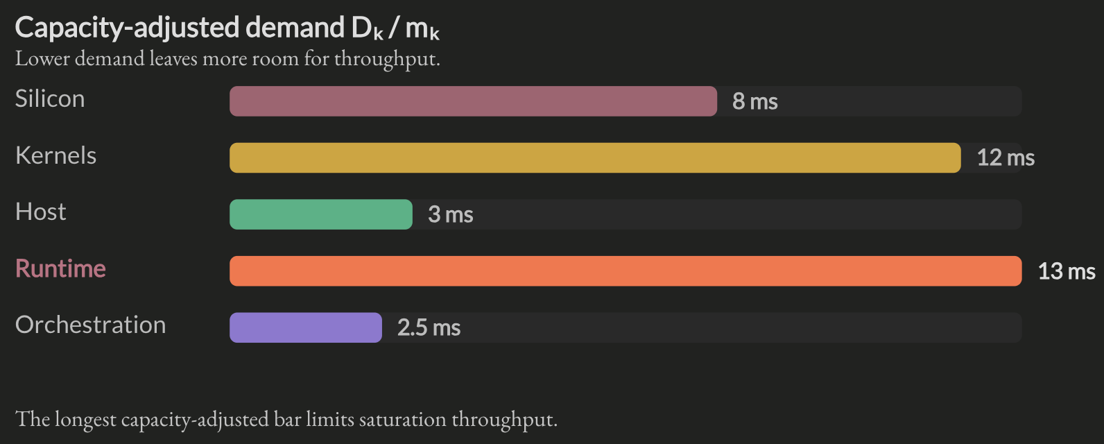
Demand alone is not enough to compare layers. A resource pool with more equivalent capacity can handle more work than one with the same demand and fewer resources. Let $m_k$ represent the equivalent parallel capacity assigned to modeled resource center $k$. Adding equivalent inference-server replicas can increase the aggregate capacity of every per-replica service center represented in the model, when $D_k$ is measured per replica. It does not automatically increase the capacity of shared routers, networks, caches, or tensor-parallel groups. A larger replica pool can also change routing demand through cache locality, load imbalance, cross-replica transfers, and cache misses. The map below compares capacity-adjusted demand, $D_k / m_k$, before the next section formalizes the bound.
The initial values are illustrative rather than measurements from one production system:
| Layer | $V_k$ | $S_k$ | $m_k$ | Why this baseline is reasonable |
|---|---|---|---|---|
| Silicon | 1 | 8 ms | 1 | One modeled accelerator phase with a meaningful memory-movement cost. Decode-heavy serving often makes weight or KV-cache movement a major part of the accelerator demand. |
| Kernels | 4 | 3 ms | 1 | Four representative kernel stages produce 12 ms of demand. Kernel shape, padding, occupancy, fusion, and memory movement commonly make this layer a close competitor to the runtime. |
| Host | 3 | 2 ms | 2 | Several scheduling, dispatch, or transfer stages run through an effectively parallel CPU pool. This keeps host work secondary for an isolated single-node baseline while leaving room for NUMA, contention, and transfer changes to expose it later. |
| Runtime | 2 | 6.5 ms | 1 | Two modeled runtime passes, such as prefill and decode, produce 13 ms of demand. Batching, KV-cache management, and model-specific scheduling often make the runtime the first bottleneck. |
| Orchestration | 1 | 2.5 ms | 1 | One routing decision has modest local service time. Its capacity is one because downstream replica count does not automatically mean that the router has equivalent parallel workers. Its larger effects usually appear through cache misses, imbalance, and extra downstream work. |
This produces illustrative capacity-adjusted scores of 8 ms, 12 ms, 3 ms, 13 ms, and 2.5 ms. Runtime starts as the raw-capacity bottleneck, with kernels close behind. A 10% runtime improvement changes 13 ms to 11.7 ms, so kernels become the next raw-capacity bottleneck. These rows are optimization-domain scores until measured work has been assigned to distinct resource centers. Orchestration represents router-local work here. In real deployments, its larger effects often appear indirectly through downstream visits, cache hits, replica balance, and service times, although a centralized router can also become a direct bottleneck.
This map is a first-order model, not a trace of every execution. In practice, $V_k$, $S_k$, and $m_k$ are estimated from traces, counters, microbenchmarks, and whole-system measurements. The model is useful because it makes assumptions visible and provides a common way to compare optimization opportunities.
Ranking Bottlenecks
As a first-order approximation, the serving path can be represented as an open queueing network with distinct service centers and expected service demands ($D_k = V_k \cdot S_k$). A service center is a modeled resource pool that processes work independently, such as a GPU, CPU worker pool, network link, or router. The five layers are optimization domains, so this bound applies only after their measured work has been mapped to distinct resource centers. Goodput can be lower because requests that violate latency, quality, or resource constraints do not count as useful completed work. In a simplified model where every service center has the same capacity, and $D_{\max} = \max_k D_k$, the raw capacity bound becomes:
$$ \lambda_{\text{capacity}} = \frac{1}{D_{\max}} $$
More generally, if resource center $k$ has capacity $m_k$, the ideal capacity bound is $\lambda_{\text{capacity}} \leq \min_k(m_k / D_k)$. Use seconds for $D_k$ to obtain requests per second. If service times are shown in milliseconds, multiply the result by $1{,}000$. A single GPU or tensor-parallel GPU group is usually modeled as $m_k = 1$ when its demand is measured as service time for that group. Bandwidth-limited resources need an equivalent capacity unit rather than a literal worker count. Achieved throughput can be lower because of blocking, synchronization, imbalance, cache effects, transfer limits, overlap constraints, and SLO requirements. This is a multi-center queueing approximation, not a one-dimensional max-flow problem. The bottleneck is the resource center with the highest normalized demand $D_k / m_k$, not necessarily the largest raw $D_k$.
This gives the first rule for optimization: estimate demand before changing code, then evaluate the change against the goodput objective and its SLO constraints. If a routing policy creates three modeled prefill stages for a request, reducing the service time of one decode kernel may have less impact than eliminating one of those stages.
Queueing changes the return
The Mean Value Analysis (MVA) method provides a way to estimate response time and queue lengths for a specified queueing-network model with known service demands, visit ratios, and client population. It motivates why a local service-time change can alter queue wait elsewhere, while whole-system benchmarks measure the actual effect in an inference deployment.
The effect is not linear because faster service changes queue lengths and arrival patterns. A faster prefill stage can change the number of requests admitted to decode when the runtime is admission- or queue-limited. A faster router can send work to a device that is already saturated if its routing signal does not include current load. The right comparison is the end-to-end response time under target concurrency, not the isolated speedup of the modified component. A subsystem microbenchmark tests whether the local hypothesis is reasonable. The whole-system benchmark determines whether that change improves the serving path under the workload and SLOs that matter. Variability injected by upstream layers also inflates waiting time downstream. Kingman’s approximation captures this effect. In the formula, $C_a$ is the coefficient of variation of inter-arrival times (the standard deviation divided by the mean), and $C_s$ is the coefficient of variation of service times. They are normalized standard deviations, not variances themselves.
$$ W_q \approx \frac{\rho}{1 - \rho} \cdot \frac{C_a^2 + C_s^2}{2} \cdot S $$
This connects directly to the Pollaczek–Khinchine formula , which we use for an $M/G/1$ queue:
$$ W_q = \frac{\rho \cdot S}{1 - \rho} \cdot \frac{1 + C_s^2}{2} $$
The two equations have the same structure. The P-K formula assumes Poisson arrivals, whose inter-arrival coefficient of variation is $C_a = 1$. Substituting that value into Kingman’s equation gives the P-K variance multiplier $(1 + C_s^2) / 2$. Kingman adds the $C_a^2$ term so the model can also represent bursty or unusually regular arrivals. This is why reducing service-time variance and smoothing upstream arrivals can both improve queue wait, even when their average amount of work is unchanged.
An optimization that lowers average service time but increases variance can make the tail worse.
Choosing the next experiment
The next experiment should stay inside the feasible goodput region. A change that improves raw throughput while violating TTFT, TPOT, quality, or resource constraints is not an improvement to the serving objective. Rank candidates by measured demand, end-to-end sensitivity, expected local gain, confidence in the measurement, implementation risk, and cost. Here, the important rule is simple: choose a small experiment that can validate or disprove the current bottleneck hypothesis, then rerun the whole-system benchmark.
Studying Full-Stack Inference Providers
Disclosure: I have no affiliation with any of the companies discussed here. This section is an independent, constructive analysis of their publicly available engineering posts. The goal is to learn where they find optimization opportunities and relate those choices to the full-stack view developed in this article. Performance figures remain attributed to their original sources, with the scope and measurement context stated by those sources.
Makora and Baseten provide complementary case studies for the layered model. Makora’s homepage describes optimization agents for orchestration, serving engines, algorithmic strategies, GPU kernels, and heterogeneous hardware. Baseten’s GLM-5.2 engineering post describes a production path that combines runtime changes, quantization, routing, disaggregation, and speculation. Studying these examples helps show how inference optimization can be approached across the full stack, where a change in one layer can depend on or expose opportunities in another.
Makora reports “up to 5x” throughput uplift and “up to 70%” lower time to first token on its homepage. These are company-reported upper bounds. A public number deserves the same scrutiny as any other benchmark: the model, hardware, quantization, prompt and output lengths, concurrency, baseline, metric, and measurement method all need to be visible. The Artificial Analysis provider benchmark for GLM-5.2 is an example of an outside measurement that includes the workload and methodology context, and it currently lists both Makora and Baseten as providers. It provides a defined comparison point for public endpoints without establishing Makora’s homepage maximums. Each company’s technical posts provide the primary detail for its own experiments, so their numbers should remain attributed to the original source and scoped to the stated workload.
Makora: Several layers move together
In TrainSpotting , Makora describes optimizing Qwen3.5-4B, Qwen3-30B-A3B, and Gemma4-31B on AWS Trainium2. The serving path uses vLLM-Neuron , so the work spans the accelerator, compiler and framework path, serving runtime, and custom kernels.
For Qwen3.5-4B, Makora packs recurrent and convolutional state to reduce DMA waste, pads a projection to match Trainium2’s 128-wide tiles so the compiler can pipeline it, and fuses a dependent decode path to keep intermediate state in SBUF. For Qwen3-30B-A3B, it adds selective expert decode, on-device sampling, and EAGLE-3 speculative decoding. For Gemma4-31B, it enables a fast attention path, changes the KV transfer block size, and fixes redundant work in sliding-window attention.
Makora reports 1.4x to 6.8x speedups relative to the default vLLM-Neuron path across these models. The details matter more than the headline. The gains come from matching model shapes, compiler behavior, memory movement, and serving policy to the target hardware. This is a broad optimization opportunity: move from generic defaults to a measured baseline that matches the model and the hardware serving it. That baseline gives later kernel, runtime, and orchestration changes a meaningful starting point.
Its Gemma 4 case study shows the GPU version of the same pattern: a low-occupancy verification kernel is changed with split-KV, then a trained DSpark draft head improves accepted length. The post reports a 6x kernel improvement and up to 82% end-to-end throughput improvement for the complete setup. These figures illustrate the model while remaining company-reported benchmarks.
Baseten: One model, several layers
Baseten is another provider in the Artificial Analysis GLM-5.2 comparison with a useful public engineering case study. In How we built the world’s fastest API for GLM-5.2 , Baseten attributes its reported 280-plus tokens per second to several changes across the stack: a customized runtime for the model’s shared DSA weights, in-house NVFP4 quantization for Blackwell GPUs, KV-aware routing with NVIDIA Dynamo, prefill/decode disaggregation, and Multi-Token Prediction heads.
The case study maps directly onto the article’s layers. Runtime and model adaptation reduce the work needed for the new architecture. Quantization changes the representation and the hardware path. KV-aware routing changes which replica receives a request. Disaggregation separates prefill and decode so each can be provisioned and tuned for its own workload. Multi-Token Prediction changes how many target-model steps are needed. The result is a useful example of why an end-to-end improvement can require coordinated changes across several subsystems.
For its observed workload shapes, Baseten reports that disaggregation produced 2x higher tokens per second, and that the overall endpoint reached more than 280 tokens per second as measured by Artificial Analysis. These figures describe Baseten’s configuration rather than a universal result. The collaboration between the runtime, routing, network, and hardware choices is the main lesson for this article.
The case studies show why the stack map needs a repeatable measurement loop. Searching efficiently means turning those observations into experiments that can confirm where the current demand and capacity constraints actually are.
Searching Efficiently
An efficient search cycle keeps the workload definition, the end-to-end measurement, and the layer-level explanation connected. The summary is:
| Phase | Evidence to collect | Decision it supports |
|---|---|---|
| Defining the workload | Model, hardware, precision, prompt and output distributions, concurrency, quality constraints, and SLOs | Which goodput objective and operating region matter |
| Measuring the baseline | TTFT, TPOT, throughput, goodput, queue time, memory use, utilization, and tail percentiles | How the complete serving path behaves before a change |
| Mapping work to layers | Router logs, runtime traces, host profiles, accelerator profiles, and kernel counters | Estimates of $V_k$, $S_k$, $D_k$, variance, and capacity for each subsystem |
| Ranking bottlenecks | Normalized demand $D_k / m_k$, queueing effects, and end-to-end sensitivity | Which subsystems are likely sources of the current bottleneck |
| Choosing an experiment | Expected improvement, confidence, correctness risk, operational complexity, and cost | Which change has the highest expected end-to-end return |
| Validating the whole system | The same workload at target concurrency, with quality and resource checks | Whether the change improves goodput and remains worth keeping |
| Recomputing the model | New traces and measurements after the change | Where the bottleneck moved and which experiment comes next |
The comparison stays end to end. A microbenchmark tests whether a local hypothesis is reasonable. The whole-system benchmark determines whether that local improvement changes goodput under the workload and SLOs that matter. Synthetic workloads should be rerun as the model, runtime, hardware, routing policy, or traffic distribution changes, because each change can alter the subsystem that limits the system next.
The goal is a repeatable search for the highest expected return across the stack. The best experiment is the smallest one that can change the demand map, improve the target objective, or disprove the current bottleneck hypothesis.
This article was written with the help of Codex.