In performance engineering, every computing system—from an embedded microcontroller to a globally distributed cloud database—is fundamentally characterized by three interdependent physical dimensions: Latency, Throughput, and Resource Utilization.

Understanding how these three metrics interact through queuing theory is essential for capacity planning, designing resilient architectures, and diagnosing production bottlenecks.

Latency ($L$)

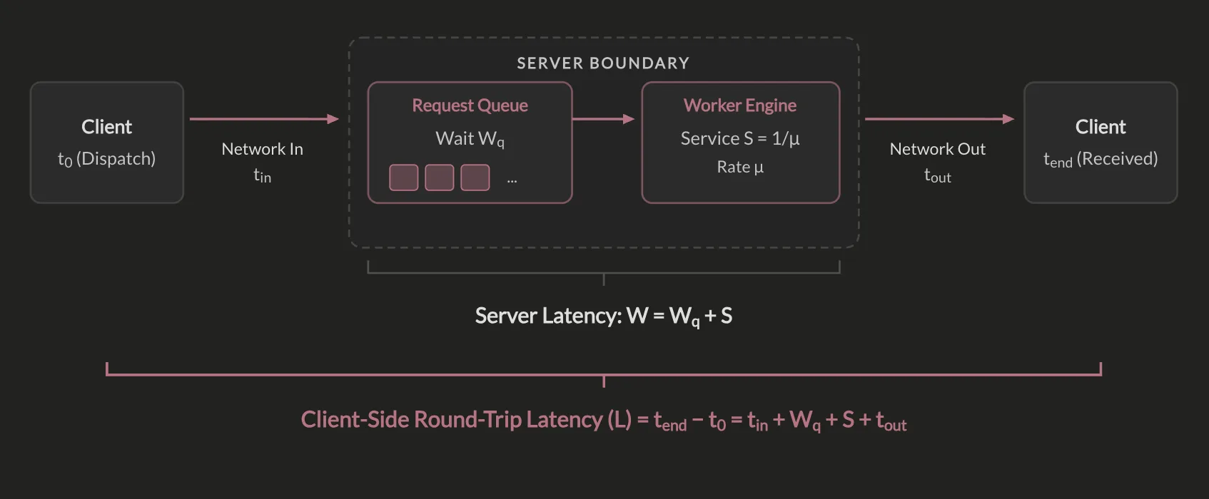
Latency measures the elapsed time required to process a request transaction. It is formally observed from two distinct system boundaries:

• Client-Side Round-Trip Latency ($L = t_{\text{end}} - t_0 = 2 \cdot t_{\text{net}} + W_q + S$): Measures the complete end-to-end user experience, including network transport ($2 \cdot t_{\text{net}}$), queue waiting delay ($W_q$), and raw server processing time ($S$).
• Service Time ($S = 1/\mu$): The time a worker spends actively executing a single request. $\mu$ is the worker’s processing rate (e.g. if a worker handles $\mu = 100\text{ req/s}$, each request takes $S = \frac{1}{\mu} = \frac{1}{100}\text{ s} = 0.01\text{ s} = 10\text{ ms}$).
• Server Latency ($W = W_q + S$): Total time spent inside the server boundary (queue wait $W_q$ + active execution $S$). When there is no queue ($W_q = 0$), latency reaches the theoretical minimum floor ($W = S = 1/\mu$).
• Tail Latency Percentiles: Evaluating mean latency hides catastrophic outliers. Systems monitor percentiles:
  • $P_{50}$ (Median): Representative baseline user experience.
  • $P_{95}, P_{99}, P_{99.9}$ (Tail Latency): High-percentile outliers driven by garbage collection pauses, worker pool starvation, TCP retransmissions, or database lock contention.

Throughput ($\lambda$ / RPS / QPS)

Throughput measures the rate of completed discrete, atomic requests per unit of time ($\lambda = \frac{N_{\text{completed}}}{\Delta t}$, e.g. Requests Per Second):

• Throughput vs. Concurrency: Concurrency ($N_{\text{in-flight}}$) is the count of requests currently in the system, whereas Throughput ($\lambda$) is the rate of requests exiting per second ($N_{\text{completed}} / \Delta t$).

Little’s Law & In-Flight Concurrency ($N = \lambda \cdot W$)

For any stable queuing system, average in-flight concurrency ($N_{\text{in-flight}}$) is strictly the product of throughput ($\lambda$) and average response latency ($W$):

$$N_{\text{in-flight}} = \lambda \cdot W$$

Little’s Law is remarkably powerful because it holds true regardless of the underlying arrival distribution, service time distribution, or queuing order. In production systems engineering, it is the primary mathematical tool for sizing infrastructure limits:

• Sizing Connection & Worker Thread Pools: If an API handles $\lambda = 1,000\text{ RPS}$ and downstream database queries take an average response time of $W = 50\text{ ms} = 0.05\text{ s}$, the number of concurrent database connections required to sustain that load without queuing is: $$N_{\text{connections}} = 1,000\text{ req/s} \times 0.05\text{ s} = 50\text{ concurrent open connections}$$
• Understanding Cascading Exhaustion: If a database lock contention or slow query causes latency to spike from $50\text{ ms} \to 500\text{ ms}$ ($0.5\text{ s}$), maintaining that same $1,000\text{ RPS}$ throughput suddenly requires: $$N_{\text{connections}} = 1,000\text{ req/s} \times 0.5\text{ s} = 500\text{ active connections}$$ If the connection pool was capped at $100$, the pool instantly exhausts, incoming requests block in queues, and upstream services fail. Little’s Law explains why downstream latency degradation directly triggers upstream connection and thread starvation.
• Calibrating Load Tests: When configuring load testing tools (wrk, k6, locust), generating a target throughput $\lambda$ at expected latency $W$ requires configuring exactly $N = \lambda \cdot W$ concurrent virtual users (VUs).

Resource Utilization ($\rho$)

Resource utilization measures the fraction of total available processing capacity actively executing requests over an observation time window $\Delta t$:

$$\rho = \frac{\sum_{i=1}^c T_{\text{busy}, i}}{c \cdot \Delta t} = \frac{\lambda}{c \cdot \mu}$$

At any single instant $t$, a worker core is in a binary state (either computing or idle). Therefore, utilization is fundamentally a time-integrated metric—evaluating the cumulative busy seconds across all $c$ cores divided by the total available core-seconds ($c \cdot \Delta t$) within the observation window. In the steady-state long run with arrival rate $\lambda$ and service rate $\mu$, this empirical time-average converges to the theoretical load $\rho = \frac{\lambda}{c \cdot \mu}$.

To understand how this formula works:

• Arrival Rate ($\lambda$): The incoming demand (e.g. $150\text{ req/s}$).
• Service Rate per Core ($\mu$): How many requests a single worker core can process per second (e.g. $\mu = 100\text{ req/s}$, which means each request takes $S = \frac{1}{\mu} = \frac{1}{100}\text{ s} = 0.01\text{ s} = 10\text{ ms}$ to execute).
• Total Cluster Capacity ($c \cdot \mu$): The maximum throughput achievable across all $c$ parallel worker cores (e.g. $c = 2\text{ cores} \times 100\text{ req/s} = 200\text{ req/s}$).
• Utilization ($\rho = \frac{\text{Demand}}{\text{Capacity}} = \frac{\lambda}{c \cdot \mu}$): The proportion of capacity in use (e.g. $\frac{150\text{ req/s}}{200\text{ req/s}} = 75%$).

• Under-Utilized ($\rho < 0.5$): Workers frequently idle. Incoming requests find an idle worker immediately with near-zero queue wait ($W_q \approx 0$), achieving the theoretical minimum latency floor ($W \approx S = 1/\mu$), but hardware infrastructure is under-utilized.
• Operational Knee ($\rho \approx 0.7 - 0.8$): The sweet spot balancing high hardware efficiency with sufficient buffer headroom ($1 - \rho \approx 20%\text{–}30%$) to absorb traffic bursts without queue buildup.
• Saturation Limit ($\rho \to 1.0$): Worker duty cycles reach 100%. Incoming requests find all servers occupied, causing queue wait times ($W_q$) to explode asymptotically toward infinity.

Live Simulation: Stochastic Queuing & Utilization

The interactive simulation below generates stochastic Poisson request arrivals ($\lambda$) and processes them across $c$ parallel worker cores with exponential service times ($\mu$).

Use the preset buttons or sliders to dynamically observe the three utilization regimes in real time:

Diurnal Traffic Cycles & Autoscaling Dynamics

In real production systems, arrival rate $\lambda(t)$ is rarely constant. User traffic naturally ebbs and flows across a 24-hour diurnal cycle—reaching a quiet low-traffic period at 3 AM and surging during peak business hours around 2 PM.

How capacity is provisioned against this wave presents a fundamental engineering trade-off:

• Static Provisioning (Fixed Cores): Provisioning a fixed worker pool leaves machines idle with low utilization ($\rho \approx 15%$) at night, wasting infrastructure spend, while peak afternoon spikes overwhelm the fixed capacity ($>100%$ load), triggering catastrophic queue buildup and tail latency ($P_{90}$) breaches.
• Reactive Autoscaling (Elastic Capacity): An autoscaler dynamically scales out worker instances during morning ramps and scales in during late-night low-traffic periods to hold utilization near a healthy target ($\rho \approx 70%$).

The simulation below demonstrates this 24-hour diurnal wave. Toggle between Static and Autoscaling strategies or scrub through the day to observe how elasticity absorbs traffic spikes without queue buildup and tail latency spikes:

Summary

This note and its interactive queuing simulation engines were co-authored in pair programming with Antigravity (Agy) .