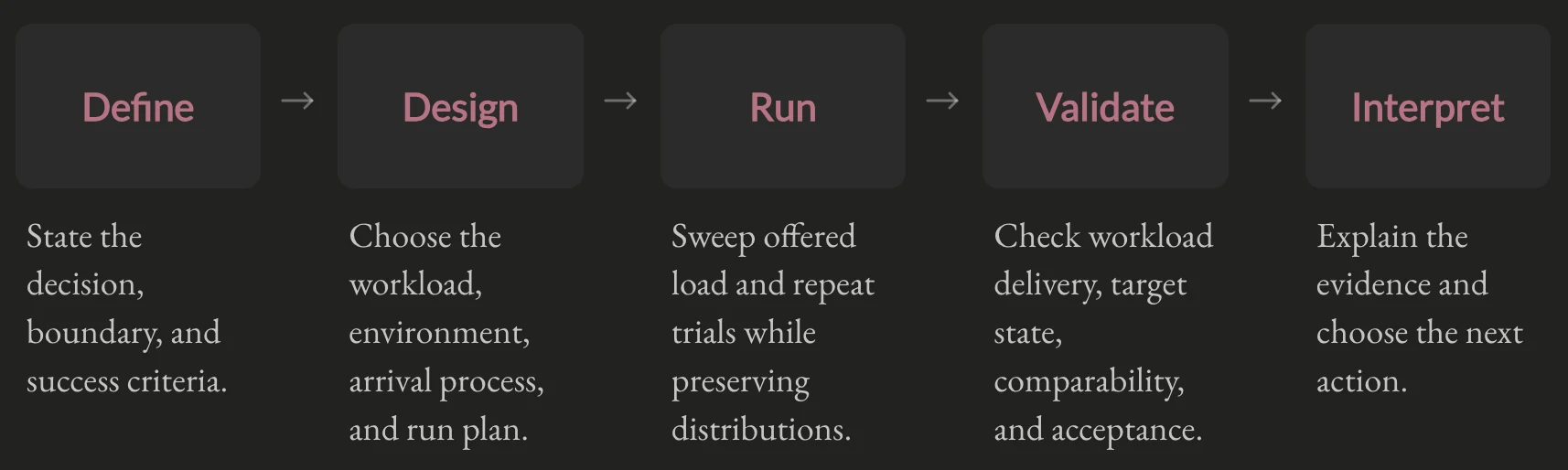


Benchmark results are evidence about a system under a particular workload and measurement procedure. A report claiming “p99 latency of 12ms at 5,000 req/s” is useful only if it helps answer a decision such as whether to launch, scale, or change the system. The same applies to an LLM benchmark that reports 30ms p99 TTFT for fixed 128-token prompts while production sends 4,000-token conversations.
An SRE starts with the service level that users need, then chooses indicators and experiments that measure it. Google’s SRE guidance treats latency, traffic, errors, and saturation as complementary signals. It recommends percentile latency indicators over averages when the tail matters, and its SLO guidance treats targets as service- and workload-specific rather than universal constants.
The practical output is a short benchmark brief before the run and a result report after it. The brief records the objective, workload, measurement boundary, environment, and expected failure behavior. The report records the SLO result, offered and achieved load, latency distribution, resource saturation, and what happened beyond the tested boundary.
By the end of this article, you should be able to turn a production question into a benchmark, recognize when its measurements are invalid, and explain what the result does and does not establish.
Defining the Benchmark
The benchmark starts with a performance problem statement. State the decision the measurement should support, the user-visible outcome that matters, the workload and system boundary, and the evidence that prompted the work. The statement should also say what result would change the decision. The load-generator setup comes later.
Brendan Gregg’s Performance Analysis Methodology provides the starting questions: what makes us think there is a performance problem, has the system performed well before, what changed, how does the problem appear in latency or runtime, who is affected, and what environment is involved. For benchmark work, add the suspected limiter, the baseline, the metric to improve, and the constraints that must remain true. Gregg’s benchmarking checklist adds practical checks such as asking why the result is not twice as good, whether the system was tuned, whether the benchmark measured the intended behavior, and whether the result matters.
Benchmarking and optimization form one loop . Run a representative workload, verify that it exercises the intended path, inspect the system while it runs, identify the limiting resource or queue, and estimate whether changing it is worth the cost. Then change the implementation or configuration and rerun the benchmark. For example: can a new batching policy reduce time to first token for this request mix while preserving output quality, error rate, GPU memory limits, and the existing user-facing SLO? A useful benchmark makes that payoff and those boundaries explicit, even when the result is that the proposed change is not worth pursuing.
Writing the Performance Problem Statement
| Question | Answer before the benchmark |
|---|---|
| What decision are we making? | Launch readiness, regression, tuning, or overload behavior. |
| What evidence started the investigation? | An observation, alert, complaint, trace, baseline, or forecast. |
| Has the system met the expectation before? | The previous version, configuration, traffic level, or known baseline. |
| What changed or is expected to change? | Software, hardware, workload, traffic, model, configuration, or topology. |
| Who or what is affected? | Customer journey, request class, latency or runtime symptom, errors, and correctness impact. |
| What workload is in scope? | The actors, request classes, phases, expected demand, and important exclusions. |
| Where is the boundary? | Client or server measurement point, dependencies, versions, topology, and resource limits. |
| What might be limiting? | A resource, queue, dependency, or software limit, plus signals that could confirm or reject it. |
| What counts as success? | The SLI, SLO, time window, and intended overload behavior. |
A benchmark-ready statement can follow this shape:
We are evaluating [decision] for [customer journey or system outcome]. Under [workload and offered demand], [system version and environment] must achieve [SLI/SLO] at [measurement boundary]. We will vary [factors], observe [limiter signals], and consider the result valid when [acceptance and overload criteria] hold.
The SLI is the measurement. The SLO is the target. Google SRE’s SLO guidance recommends connecting the target to the service users’ experience. The threshold, request population, measurement boundary, and window must be explicit before the load level is chosen.
At light load, observed response time approaches the uncontended response-time floor $W_0$. It approximates service time $S$ only when the measurement boundary isolates that service center and excludes other latency such as network transfer, serialization, runtime overhead, and dependencies. Use the floor as a diagnostic reference while keeping the user-visible SLO as the objective. If the statement names a suspected limiter, observe it while the benchmark runs. Gregg’s USE Method provides a compact check for utilization, saturation, and errors across relevant hardware and software resources.
The rest of the article follows from this statement. We design the benchmark and workload, run the experiment, check that the measurements are valid, and interpret the result.
Designing the Benchmark and Workload
The problem statement defines the workload’s scope. Designing the benchmark turns that scope into a model of demand, a system boundary, an arrival process, and a repeatable run plan. Theory gives us the dimensions to preserve. Practice determines which values and variations represent the system that users actually experience.
Defining the Workload
Synthetic load becomes useful when it preserves the parts of the system that determine customer-visible behavior:
| From the problem statement | Benchmark representation | Validate with |
|---|---|---|
| Request classes and user journeys | Separate scenarios, SLOs, and mix weights. | Domain experts and user-impact data. |
| Request cost and execution phases | Distributions of query shape, prompt and output length, read/write mix, and prefill/decode ratio. | Production traces and service-time measurements. |
| State that changes the cost | Hot and cold keys, prompt-prefix reuse, cache eviction, working-set size, and memory pressure. | Cache metrics, data distributions, and representative state. |
| Arrival behavior | Arrival schedule, concurrency, bursts, retries, and admission behavior. | Production traces or a justified stochastic model. |
The performance engineer and domain experts should co-author the entire benchmark cycle, including the problem statement, workload, run design, validation, and interpretation. The performance engineer contributes measurement discipline and a repeatable setup. Domain experts ensure that the scenarios and success criteria represent outcomes customers actually care about. The benchmark should record those assumptions so a later change in traffic or product behavior is visible in the result.
Designing the Environment Under Test
The target service is only one part of a benchmark. The benchmark also includes resource allocation, execution state, request paths, placement context, and the measurement harness. Start by deciding which of these belong to the question and which should be held constant.
An end-to-end benchmark keeps an external dependency in the test when its capacity, latency, retries, or errors are part of the user-visible outcome. A component benchmark can mock or stub that dependency when its variability would hide the behavior under study. The replacement should preserve the interface, payload sizes, timing range, failure behavior, and backpressure that matter to the experiment. Record the boundary so a component result is not mistaken for an end-to-end result.
In practice, the same setup can produce different measurements because a network path changes between availability zones, a workload lands on different hardware, or a noisy neighbor causes an outer hypervisor to give the workload less scheduling time. These effects can be controlled, measured as workload dimensions, or isolated with a controlled replacement. The choice belongs in the benchmark plan.
Repeated trials estimate run-to-run variation, but they do not make systematic differences between zones, hardware pools, or placement conditions disappear. Stratified reporting is the default: record the stratum for each run and report metrics and constraints per stratum before combining results. Use normalization only when the comparison requires a common reference and an independently validated calibration model exists for the workload and operating range. Report raw values alongside normalized values so the adjustment cannot hide a real system difference.
Defining the Run
The experiment plan defines how the system reaches the state being measured and how the measurement window is selected:
- Warm-up and initialization: Run the target workload until initialization, compilation, connection pools, caches, and inference memory pools reach the state that the measurement is meant to represent. Record the warm-up interval, but do not mix it with steady-state results.
- Load transitions: Decide whether each load point begins as an independent trial or intentionally inherits state from the previous point. Independent trials should drain work, reset the required state, and warm up again. A continuous ramp is appropriate when backlog, recovery, or state carried between load levels is part of the behavior under study.
- Steady-state measurement: Record high-resolution latency distributions and resource metrics for long enough to cover the relevant periodic behavior, such as garbage collection, database checkpoints, autoscaler actions, or inference cache churn. The duration is an experimental parameter, not a universal constant.
- Cooldown and reset: Reduce traffic in a controlled way, drain in-flight work, and check for leaks, unclosed connections, errors, and other state that could contaminate the next independent trial.
The arrival process is another workload input. Closed and open workload models explain whether the generator is bounded by outstanding responses or sends requests at an independent rate. Use a closed-loop generator when the benchmark represents a bounded population that waits for responses. Use an open-loop schedule when the question concerns a fixed offered rate, pauses, or backlog. The queueing article’s discussion of arrival processes gives more intuition for how those arrivals create waiting. The schedule should come from the traffic pattern being studied, and the measurement must preserve requests that were supposed to arrive while the service was busy.
Coordinated Omission
When the intended workload is open-loop, a response-dependent generator can wait for each response before sending the next request. During a server pause, it then omits arrivals that should have entered the system and reports latency only for the requests that were eventually sent. This is Coordinated Omission, a measurement flaw described by Gil Tene in How NOT to Measure Latency . Response-dependent generation remains valid when the benchmark intentionally models a bounded population whose next request depends on a previous response.
For a fixed-rate benchmark, record the scheduled arrival, actual dispatch, service start when observable, and completion. Generator-side dispatch delay is the interval between scheduled arrival and actual dispatch. Target-side queue wait is the interval from arrival at the target to service start. Report response time from scheduled arrival to completion so a server pause remains visible in the latency distribution. Gil Tene’s article covers more detailed correction methods.
Recording the Design
Write the experiment plan down before running it. Record the exact system and generator versions, configuration, workload seed, offered load, warm-up and steady-state boundaries, expected resource limits, dependency setup, and conditions that invalidate a trial. During each steady-state window, record the latency distribution, achieved load, errors, dropped work, generator resource usage, and infrastructure changes. The execution should follow this plan closely enough that a later result can be compared with the baseline.
Running, Validating, and Interpreting the Benchmark
Run the plan exactly as written. Running produces measurements, validation selects the measurements that can support a comparison, interpretation explains the observed behavior, and reporting connects the evidence to a decision.
Running the Experiment
A rate sweep should vary offered load across the range relevant to the user objective and record both SLO compliance and resource behavior. Use multiple steady-state windows at each load, include the request mix defined by the problem statement, and stop or continue based on the risk of the test.
The useful result is a curve of offered load, achieved load, SLO compliance, latency distribution, errors, and resource saturation. Mark the highest repeatedly passing tested point and report the sweep resolution and run-to-run spread. The resulting boundary applies to the sampled load points and their resolution. There is no source-backed universal utilization knee or required multiplier.
- Replication: Write the stopping criterion into the experiment plan. Repeat trials until the uncertainty or spread is stable enough for the decision, then report that spread. The number of trials depends on variability and decision risk, not a universal minimum.
- Raw distributions: Preserve a histogram for every trial and report between-trial variation. Merge histograms only when weighting trials by their event counts matches the question being answered, and state that weighting explicitly. Do not average percentile values.
- Baseline vs. contention: Use light-load distributions to estimate the uncontended response-time floor and target-load distributions to characterize queueing. Do not use the minimum observation as the SLO.
- Regression decisions: Compare SLO compliance and confidence or spread, not only a single percentage improvement.
Validating the Evidence
Before comparing configurations, check that each trial produced the workload and system state described in the benchmark plan. A small stall experiment can also reveal whether the load generator preserves scheduled arrivals when the target stops responding temporarily.
| Validation area | What to establish | Evidence to record |
|---|---|---|
| Offered workload | The intended schedule and rate reached the target without the generator becoming the bottleneck. | Scheduled arrivals, actual dispatches, generator-side dispatch delay, generator resource usage, and dropped work. |
| Target state | The measurement window represents the intended steady state rather than warm-up or cooldown. | Initialization state, warm-up boundary, latency distribution, achieved load, errors, timeouts, and cancellations. |
| Run comparability | Environment and placement differences are recorded before results are combined. | Zone, hardware pool, placement, infrastructure changes, and other environment strata. |
| Trial acceptance | The run contains enough complete evidence to support the comparison. | Acceptance criteria from the experiment plan and the reason for excluding any run. |
Repeated trials estimate run-to-run variation, but they do not remove systematic differences between environments. Compare metrics and constraints within each stratum before combining results. Exclude trials with dropped work, generator-side dispatch delay beyond the configured tolerance, incomplete warm-up, generator saturation, unrecorded placement changes, or missing error and completion data. Preserve target-side queueing and completion delay because those can be the behavior under study.
Interpreting the Evidence
A valid benchmark result is useful when it explains both the observed service level and the conditions that produced it. The highest repeatedly passing tested point is a result boundary whose scope is limited to this workload, configuration, sweep resolution, and observed run-to-run variation.
Queueing models from Queuing Theory for Systems Engineers provide vocabulary for the explanation, but the benchmark should start with the end-to-end result:
| Signal | What to compare | What it helps explain |
|---|---|---|
| SLO compliance | Good-event fraction, latency percentiles, errors, and correctness. | Whether the user-facing objective held. |
| Offered and achieved load | Intended arrivals versus requests the system actually received and completed. | Whether the generator or target limited the experiment. |
| Request distribution | Request classes, service times, payload sizes, phases, and cache state. | Which work produced the latency distribution. |
| Resource evidence | Utilization, saturation, errors, queues, and software limits. | Which subsystem limited the result. |
| Run validity | Warm-up state, generator-side dispatch delay, dropped work, and repeated-trial spread. | Whether the result is comparable and trustworthy. |
| Boundary behavior | Queue growth, shedding, retries, timeouts, cancellation, and recovery. | What the system does when the objective stops holding. |
For an inference service, scheduler, GPU, KV-cache, network, and dependency metrics can explain the end-to-end result without pretending that the entire engine is one exact queue. The useful conclusion is a chain of evidence from the customer-visible symptom to the subsystem behavior that produced it.
Reporting the Decision
A benchmark report assembles the outputs of the design, execution, validation, and interpretation stages into one reproducible artifact:
| Report section | Include |
|---|---|
| Question and decision | The performance problem statement and the decision the evidence supports. |
| System and workload | Versions, topology, configuration, dependencies, initial state, request mix, arrival model, and offered load. |
| Run protocol | Warm-up, load transitions, steady-state window, stopping criterion, and generator limits. |
| Validity | Trial acceptance criteria, excluded runs, environment strata, and measurement limitations. |
| Results and explanation | Per-trial latency distributions, SLO compliance, errors, correctness, achieved load, resource signals, and suspected limiter. |
| Decision and next step | The supported conclusion, known limitations, and the next experiment or operational action. |
The benchmark is ready to inform a decision when its result is explained, reproducible from the recorded procedure, and bounded by its limitations.
This note was co-authored in pair programming with Antigravity (Agy) and Codex.